Notes to Instructor

Created by Atul Varma (Class of 2001, Kenyon College)

Many of us have fond childhood memories of creating wiggly lines, circles, and other doodles on the magic screen of an Etch A Sketch®, a toy that first appeared in the early 1960's. In this module, you will get the chance to relive those endless hours of etching fun through the use of parameterizations and MAPLE.

A parameterization of a curve in the plane is a pair of functions, X  =  x(t) and Y = y(t), that describe the motion of a particle in the plane. The function x(t) serves the same role as the left-hand dial on the Etch A Sketch; it describes the motion of the particle in the x-direction. The function y(t), like the right-hand dial, dictates the motion in the y-direction. At any given value of time t, the pair (x(t), y(t)) determines the particle's exact location at that time.

As you will soon discover, MAPLE's parametric plotting capabilities are more conducive to creative doodling than those familiar white dials ever were. In fact, by working through each of the sections listed below, you will learn how to draw almost anything you wish. In the final section of this project, you will then be asked to show off your new skills by creating your own elaborate doodle.

Judy Holdener is Associate Professor of Mathematics and 
Keith Howard  is Assistant Professor of Mathematics, both at Kenyon College.

Copyright © 2004 by Judy Holdener and Keith Howard

Published June, 2004

To start, consider the parameterization (x(t), y(t)) = (cos(t), sin(t)), with t varying from 0 to 2. At time t = 0, the particle is at the point (x(0),y(0)) = (cos(0), sin(0)) = (1, 0). As t increases from 0 to /2, cos(t) decreases in value from 1 to 0, and sin(t) increases from 0 to 1. Hence, for 0 t /2, the particle moves from its starting point at (1, 0) to the point (0, 1). It is not hard to see that the result is a quarter circle of radius 1 traversed in the counter-clockwise direction.

Parametric Plotter

Using the MAPLET: A MAPLET is a graphical interface that allows the user access to the power of MAPLE without interacting with the complex underlying code. The Parametric Plotter MAPLET, which can be opened by clicking the link at the right, is designed to plot parametric curves. Please be patient while the initial MAPLET loads -- you may not see any indication onscreen that anything is happening until the Java/MAPLET button appears on your tsk bar.

The MAPLET is composed of, from top to bottom, a plotter box, four text fields to enter the parametric equations and the parameter plotting range, and a sequence of buttons designed to plot a designated parametric curve, clear the last curve plotted, clear all plots, and exit the MAPLET. Upon opening the MAPLET, you will see that it has been initialized with the parameterization (x(t), y(t)) = (cos(t), sin(t)), varying t from 0 to 2. Notice that the terms in the text fields are written in MAPLE syntax. For example, 2 is entered as 2*Pi. The syntax required in all text fields must be consistent with the language of MAPLE. Thus, multiplication must be made explicit, and special functions, such as the sine function, must be written just as in the MAPLE program.

By clicking the "Plot" button, you can obtain a plot of the initialized parametric functions. To plot other parametric equations, simply make the necessary changes in the appropriate text fields. The plots of new parametric curves will overlay the plots of previous curves, unless you use the "Clear" button, which will clear all plots from the plotter, allowing you to start anew. Clicking the “Clear Last” button will erase just the most recent curve plotted. The plots produced by the MAPLET are not drawn on a one-to-one scale, thus special attention should be given to axes labeling, as images may appear slightly warped. When you are done using the Parametric Plotter MAPLET, you can close the MAPLET by clicking the "Exit" button.

NOTE: If the sizing of your MAPLET window is not optimal, and you are having difficulty seeing all of the buttons/features, then see the Notes to Instructor.

---

Exercise 2.1

1. Using the Parametric Plotter MAPLET, plot the curve parameterized by
   (x(t), y(t)) = (cos(t), sin(t)) for 0t /2, then for 0t  , and finally for 0t 3/2. What do you observe?

2. Recall that the equation of the unit circle arises from the distance formula -- all points on the circle are located at a distance of exactly one unit from the origin. Use this equation to show that all points of the form (cos(t), sin(t)) do indeed fall on the unit circle.

---

Exercise 2.2

1. Next use the MAPLET to plot the curve parameterized by (x(t), y(t)) = (cos(2t), sin(2t)) for 0t /2, then 0t  , and finally 0t 3/2. What do you observe?

2. Plot the curve parameterized by (x(t), y(t)) = (cos(t/2), sin(t/2)) for 0t /2, then 0t  , and finally 0t 3/2. What do you observe?

3. Plot the curve parameterized by (x(t), y(t)) = (cos(-t), sin(-t)) for 0t /2, then 0t  , and finally 0t 3/2. What do you observe?

4. Generalize your results from parts a) and b). How does the parameterization (cos(kt), sin(kt)) compare to (cos(t), sin(t))?

---

Exercise 2.3   

For each of a) through c), use the MAPLET to check your answer by producing the appropriate parametric plot.

1. Find a parameterization of a circle centered at the origin having radius 3.

2. Find a parameterization of a circle centered at (5, 3) having radius 3.

3. Can you figure out how to plot ellipses? Produce the plot of an ellipse centered at the point (5, 3) having a major axis of length 10 and minor axis of length 6. The major (respectively, minor) axis is defined to be the line segment serving as the largest (respectively, smallest) possible diameter of the ellipse.

---

As you know, two pieces of information determine the equation of a line -- for example, two points on the line, or a point on the line and the slope. Here we introduce a new way of describing lines using vectors and parameterizations. This description, unlike our previous methods, can be generalized to lines in space.

Consider the line through the two points (1, 2) and (3, 3). To describe this line using vectors, we first compute the displacement vector v = <2, 1>, which has its tail at (1, 2) and its head at (3, 3). This vector describes the direction of the line. The picture below (left) shows the line we seek together with this displacement vector.

Next notice that we can now produce any point on the line by adding multiples of the direction vector <2, 1> to the vector <1, 2>. In the right figure below, we illustrate how it works by adding two copies of <2, 1> to <1, 2>. In this way, we see that the point (5, 4) is on the line, because <5, 4> = <1, 2> + 2<2, 1>.

Figure 3.1. (Left) Adding the displacement vector <2, 1> to <1, 2> yields the vector <3, 3>.
(Right) Starting at (1, 2) and adding two displacements of <2, 1> will take us twice as far along the line.

More generally, note that any point on the line can be described by <1,2> + t <2, 1>, for some appropriate value of t. Negative values of t will correspond to points on the line heading in the other direction. Expanding the expression results in a parametric description of the line:

<1, 2> + t <2, 1> =  <1, 2> + <2t, t> =  <1 + 2t, 2 + t>.

That is, the equations x(t) = 1 + 2t and y(t) = 2 + t parameterize the line. Notice that setting
t = 0 produces the starting point (x(0), y(0)) = (1, 2), and if t = 1 we get (x(1), y(1)) = (3, 3). Hence we let t vary from t = 0 to t =1 to trace out the line segment from (1, 2) to (3, 3).

Parametric Plotter

---

Exercise 3.1

Use what you have just learned to find the parameterization of the directed line segment from (0,4) to (3,0). Since (0, 4) is your starting point, your parameterization (x(t), y(t)) should satisfy (x(0), y(0)) = (0, 4).

---

Exercise 3.2

Produce a plot of a right triangle having sides of length 3, 4, and 5.

---

Parameterizing functions is easy. If y = f(x), then the parametric equations x(t) = t and
y(t) = f(t) always work. (That, is you simply treat x as the parameter). For example, if you want to parametrize the graph of the function f(x) = x³ + 2x² - x + 9 from (0, 9) to (2, 23), then the parameterization is:

x(t) = t and y(t) = t³ + 2t² - t + 9, 0 t 2.

Parametric Plotter

---

Exercise 4.1

Figure 4.1 - The graph of a function

1. Find a parameterization of the function shown in Figure 4.1. [Hint: The right-most point on the graph is (5, 0).]

2. Now find a parameterization that traces out the same curve in the reverse direction.

3. Finally find a parameterization (x(t), y(t)) that satisfies x(0) = 0 and x(2) = 5.

---

Exercise 4.2

Figure 4.2 - A graph of a piecewise function

Find a parameterization of the piecewise-defined function shown in Figure 4.2. (Hint: This function can be plotted in two steps. Plot one piece on the MAPLET and then plot the other without clearing.)

In this section we will look at some very famous interesting curves, many of which may be new to you, because some of the most interesting curves are best described by parametric equations. To learn more than what is offered here, check out the Famous Curves Index at the History of Mathematics archive. Indeed, many of these curves have a long history.

Lissajous Curves

A Lissajous curve or figure is any curve from the family of curves described parametrically by the equations x(t) = sin(at) and y(t) = sin(bt), where a and b are constants. They were first studied in 1815 by Nathaniel Bowditch and later, in 1857, by the French mathematician Jules-Antoine Lissajous. Lissajous curves have applications in physics and astronomy. They are interesting curves.

Here's a plot of the Lissajous curve corresponding to a = 2 and b = 3; we denote this curve by L(2, 3).

Lissajous Plotter

---

Exercise 5.1

1. Experiment with Lissajous curves of the form L(a, 3) where a varies from 1 to 7. In other words, keep b fixed at 3, and let a vary from 1 to 7. What do you observe?

2. Next explore those Lissajous curves of the form x(t) = sin(at), y(t) = sin((a + 1)t). That is, explore the situation where the parameter b is just one unit larger than a. What happens to the Lissajous curves L(a, a+1) when a gets larger and larger? You'll want to make a fairly large to see the pattern. What do you discover? (Isn't it cool?)

---

The Cycloid

A cycloid is the curve traced by a point P on the rim of a wheel (or circle) rolling along a straight line in a plane. The parametric equations of a cycloid have the form:

x(t) = at - a sin(t) and y(t) = a - a cos(t),

where a is the radius of the wheel.

Cycloid Movie

---

The Epicycloid

Suppose now that a wheel of radius 1 rolls around the outside of a circle of radius 2. The curve traced out by a point on the rim of the smaller circle is called an epicycloid. Here's the plot of the curve.

Epicycloid Plotter

More generally, the epicycloid traced by a fixed point on a circle of radius B as it rolls around the outside of a circle of radius A is described parametrically by the equations:

x(t) = (A+B) cos(t) - B cos( [(A+B)/B] t ),
y(t) = (A+B) sin(t) - B sin( [(A+B)/B] t ).  

---

Exercise 5.2

Play around with this! Vary the values of A and B in the Epicycloid MAPLET to see how the epicycloid changes.

---

The Hypocycloid

The hypocycloid is the curve traced by a fixed point on the rim of a wheel as is it is rolled around the inside of a circle. If you have ever spent any time playing with Spirograph®, then you are already familiar with these curves. (Think about how you produced curves with Spirograph!).

The parameteric equations of the hypocycloid traced by a fixed point of a circle of radius B as it rolls around the inside of a circle of radius A are given by:

x(t) = (A - B) cos(t) + B cos( [(A - B)/B] t ),
y(t) = (A - B) sin(t) - B sin( [(A - B)/B] t ).  

Here's an example.

Hypocycloid Plotter

---

Exercise 5.3

Change the values of A and B in the preceding exercise to see what you can create.

---

Maple Leaf

Okay...maybe this curve isn't so famous. But it is very nice nonetheless. Check it out...

Maple Leaf Plotter

---

Exercise 5.4

Change the parameters in the Maple Leaf Plotter to see what other sorts of leaves you can create.

---

Now it's your turn! Download the MAPLE file linked below, and open it to produce your own masterpiece with parametric plots. Feel free to use some of the many different types of curves you have seen in this project.

This is the last part of the project. If you're curious about drawings by other students, you will find some on the next page.

   ParametricMasterpiece.mws

Additional MAPLE Resources:

If you really want to get fancy, feel free to use the additional MAPLE files provided below. They will allow you to add color and even an extra dimension to your picture. If your picture has some form of symmetry in it (for example, bilateral or rotational symmetry), then you might want to save some time by using one or more of the symmetry tools.

To fill a region:	FillingRegions.mws
To parameterize curves in three-dimensional space:	SpaceCurves.mws
To scale, reflect, rotate and translate curves:	SymmetryTools.mws

---

Scroll down to see some parametric art done by students at Kenyon College, where versions of this module have been used for instructional purposes for many years.

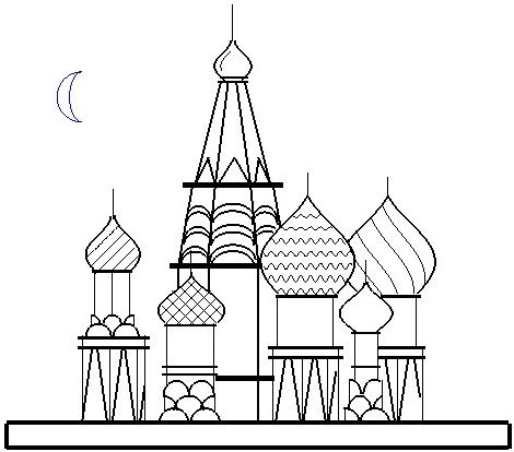
St. Basil's Cathedral -- by Nick Johnson

---

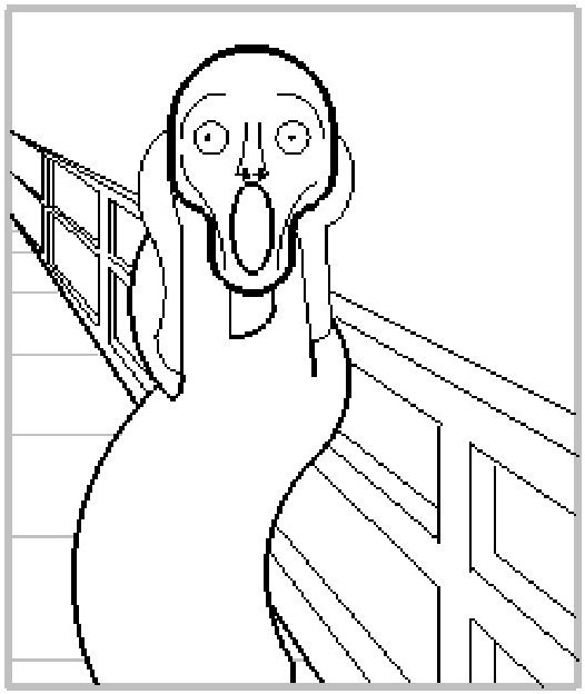
The Scream -- by Christopher Fry

---

Oh yeah? Define "Well-Adjusted" -- Christopher White

(The Calvin and Hobbes comic strip was created by Bill Watterson, a Kenyon graduate.)

---

Taj Mahal -- by David Handy

---

Are you experienced? -- by Andrew Braddock

---

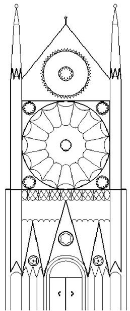
Notre Dame -- by Jenny Adams and Carolyn Wendler

---

 

Play Ball! -- by Tara Tucci

---

 

Abu -- by Laura Huss and Colin O'Brien

---

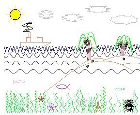
A Trip to the Islands -- by Toskhan Cooper

---

 

OH COSH! The bridge is sinking!!! -- by Lee Kennard

---

Untitled -- by Laura Jumper

---

 

Clown -- by Andrew Garstka

---

 

Pagoda -- by Atul Varma