The transport equation is a partial differential equation of the form

(1)

Here,  u  is a function of two variables   x  and  t,  and the subscripts denote partial derivatives. We will assume that  c  is a fixed constant. Given an initial condition

(2)

we would like to find a function of two variables that satisfies both the transport equation (1) and the initial condition (2).

This equation can be used to model pollution (Lehn and Scherer , undated), dye dispersion (Roychoudhury , undated), or even traffic flow (Jungel , 2002), with  u  representing the density of the pollutant (or dye or traffic, respectively) at position  x  and time  t.  For a discussion of the physical model, see Knobel (2000). For a discussion of the more general transport equation and its solutions, see Cooper (1998). For discussion and simulation of more general conservation laws, including shock wave phenomena, see Sarra  (2003).

Acknowledgment 

Components for the applet are based on David Eck's Java Components for Mathematics at Hobart and William Smith Colleges.

About the author

Joan Remski is an Assistant Professor of Mathematics
at University of Michigan-Dearborn .

Copyright 2004 by Joan Remski

Published June, 2004

Using the gradient operator 

we may rewrite equation (1) as

This equation says that the directional derivative in the  (1, c)  direction (in the  
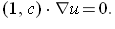
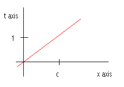
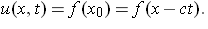
t, x-plane) is zero. So our solution  u(x, t)   must be constant in this direction. In the  t, x-plane, the  (1, c)  direction is along lines parallel to  x = ct,  which are called the characteristics of equation (1).

Now, fix a point on the  x-axis, say  (x₀, 0). The line through this point parallel to  x = ct 
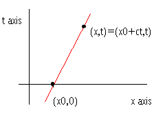
is given by  x = x₀  + ct.  Since our solution is constant along this line, we must have

 

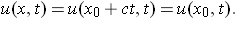
But from the initial data,

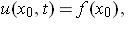
where  f  is known. So, for any  (x, t),

 

The applet on this page allows you to enter the initial data  u(x, 0)  and the slope of the characteristic lines,  c.  Press return in any of the input boxes to update the graph. Use the scroll bar beneath the graph allows to control time on the graph of the solution. Changing  c  changes the "speed" of the solution. Use the scroll bars at the top and right-hand side to control the viewpoint. 

When entering the initial condition  u(x, 0),  be sure to include * for multiplication, / for division, ^ for a power, etc. The parser also recognizes many standard math functions including  sin(x),  cos(x),  ln(x),  arctan(x), etc.

Do not leave any blank spaces in the middle of the input box.

Sample Problem

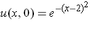
Suppose dye is spilled in a fast moving stream. Let  u(x, t)  represent the concentration of dye at  x  meters downstream from the initial spill at time  t  (measured in minutes). Suppose the initial concentration of dye at  t = 0  has the form  

and  c = 0.5.

Cooper, J. (1998), Introduction to Partial Differential Equations with MATLAB, Boston: Birkhauser.

Eck, D. (2001), Java Components for Mathematics, http://math.hws.edu/javamath/ (accessed June 17, 2004).

Jungel, A.(2002), Modeling and Numerical Approximation of Traffic Flow Problems, http://www.numerik.mathematik.uni-mainz.de/~juengel/scripts/trafficflow.pdf (accessed June 17, 2004).

Knobel, R. (2000) An Introduction to the Mathematical Theory of Waves, AMS Student Mathematical Library, Providence: American Mathematical Society.

Lehn, M., and R. Scherer (undated), Modeling of Flow and Pollution for the River Struma, http://www.mathematik.uni-karlsruhe.de/~ipm/waterman/num_modeling.html (accessed June 17, 2004).

Roychoudhury, A. (undated), Transport Processes, http://web.uct.ac.za/depts/geolsci/people/staff/roy/lectures/lec13.pdf (accessed June 17, 2004).

Sarra, S. (2003), "The Method of Characteristics with Applications to Conservation Laws," Journal of Online Mathematics and its Applications, Vol. 3, http://www.joma.org/mathDL/4/?pa=content&sa=viewDocument&nodeId=389 (accessed September 7, 2004).