The SIR Model for Spread of Disease - The Differential Equation Model
As the first step in the modeling process, we identify the independent and dependent variables. The independent variable is time t, measured in days. We consider two related sets of dependent variables.
The first set of dependent variables counts people in each of the groups, each as a function of time:
| S = S(t) | is the number of susceptible individuals, |
| I = I(t) | is the number of infected individuals, and |
| R = R(t) | is the number of recovered individuals. |
The second set of dependent variables represents the fraction of the total population in each of the three categories. So, if N is the total population (7,900,000 in our example), we have
| s(t) = S(t)/N, | the susceptible fraction of the population, |
| i(t) = I(t)/N, | the infected fraction of the population, and |
| r(t) = R(t)/N, | the recovered fraction of the population. |
It may seem more natural to work with population counts, but some of our calculations will be simpler if we use the fractions instead. The two sets of dependent variables are proportional to each other, so either set will give us the same information about the progress of the epidemic.
- Under the assumptions we have made, how do you think s(t) should vary with time? How should r(t) vary with time? How should i(t) vary with time?
- Sketch on a piece of paper what you think the graph of each of these functions looks like.
- Explain why, at each time t, s(t) + i(t) + r(t) = 1.
Next we make some assumptions about the rates of change of our dependent variables:
-
No one is added to the susceptible group, since we are ignoring births and immigration. The only way an individual leaves the susceptible group is by becoming infected. We assume that the time-rate of change of S(t), the number of susceptibles,1 depends on the number already susceptible, the number of individuals already infected, and the amount of contact between susceptibles and infecteds. In particular, suppose that each infected individual has a fixed number b of contacts per day that are sufficient to spread the disease. Not all these contacts are with susceptible individuals. If we assume a homogeneous mixing of the population, the fraction of these contacts that are with susceptibles is s(t). Thus, on average, each infected individual generates b s(t) new infected individuals per day. [With a large susceptible population and a relatively small infected population, we can ignore tricky counting situations such as a single susceptible encountering more than one infected in a given day.]
- We also assume that a fixed fraction k of the infected group will recover during any given day. For example, if the average duration of infection is three days, then, on average, one-third of the currently infected population recovers each day. (Strictly speaking, what we mean by "infected" is really "infectious," that is, capable of spreading the disease to a susceptible person. A "recovered" person can still feel miserable, and might even die later from pneumonia.)
Let's see what these assumptions tell us about derivatives of our dependent variables.
- The Susceptible Equation. Explain carefully how each component of the differential equation

(1)
follows from the text preceding this step. In particular,
- Why is the factor of I(t) present?
- Where did the negative sign come from?

(2) - The Recovered Equation. Explain how the corresponding differential equation for r(t),

(3)
follows from one of the assumptions preceding Step 4. - The Infected Equation. Explain why

(4)
What assumption about the model does this reflect? Now explain carefully how each component of the equation

(5)
follows from what you have done thus far. In particular,
- Why are there two terms?
- Why is it reasonable that the rate of flow from the infected population to the recovered population should depend only on i(t) ?
- Where did the minus sign come from?
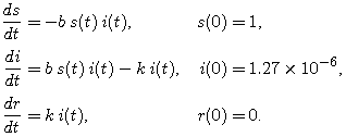
Finally, we complete our model by giving each differential equation an initial condition. For this particular virus -- Hong Kong flu in New York City in the late 1960's -- hardly anyone was immune at the beginning of the epidemic, so almost everyone was susceptible. We will assume that there was a trace level of infection in the population, say, 10 people.2 Thus, our initial values for the population variables are
| S(0) = 7,900,000 |
| I(0) = 10 |
| R(0) = 0 |
In terms of the scaled variables, these initial conditions are
| s(0) = 1 |
| i(0) = 1.27 x 10- 6 |
| r(0) = 0 |
(Note: The sum of our starting populations is not exactly N, nor is the sum of our fractions exactly 1. The trace level of infection is so small that this won't make any difference.) Our complete model is
 |
(6) |
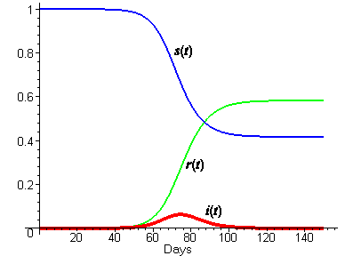
We don't know values for the parameters b and k yet, but we can estimate them, and then adjust them as necessary to fit the excess death data. We have already estimated the average period of infectiousness at three days, so that would suggest k = 1/3. If we guess that each infected would make a possibly infecting contact every two days, then b would be 1/2. We emphasize that this is just a guess. The following plot shows the solution curves for these choices of b and k.

- In steps 1 and 2, you recorded your ideas about what the solution functions should look like. How do those ideas compare with the figure above? In particular,
- What do you think about the relatively low level of infection at the peak of the epidemic?
- Can you see how a low peak level of infection can nevertheless lead to more than half the population getting sick? Explain.
In Part 3, we will see how solution curves can be computed even without formulas for the solution functions.
1 Note that we have turned the adjective "susceptible" into a noun. It is common usage in epidemiology to refer to "susceptibles," "infecteds," and "recovereds" rather than always use longer phrases such as "population of susceptible people" or even "the susceptible group."
2 While I(0) is normally small relative to N, we must have I(0) > 0 for an epidemic to develop. Equation (5) says, quite reasonably, that if I = 0 at time 0 (or any time), then dI/dt = 0 as well, and there can never be any increase from the 0 level of infection.