This module investigates a standard model of population growth in a constrained environment.

Notes for the Instructor

About this Module and its Authors

Choice of Computer Algebra System

Click on the button corresponding to your preferred computer algebra system (CAS). This will download a file which you may open with your CAS.
 

Ver. 6 or higher

Ver. 3.0 or higher

Ver. 5.1 or higher

 

Copyright 1998-2000, CCP and the authors

Published December, 2001

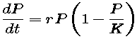
A biological population with plenty of food, space to grow, and no threat from predators, tends to grow at a rate that is proportional to the population -- that is, in each unit of time, a certain percentage of the individuals produce new individuals. If reproduction takes place more or less continuously, then this growth rate is represented by

dP/dt = rP,

where P is the population as a function of time t, and r is the proportionality constant. We know that all solutions of this natural-growth equation have the form

P(t) = P₀ e^rt,

where P₀ is the population at time t = 0. In short, unconstrained natural growth is exponential growth.

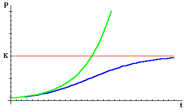
Of course, most populations are constrained by limitations on resources -- even in the short run -- and none is unconstrained forever. The following figure shows two possible courses for growth of a population, the green curve following an exponential (unconstrained) pattern, the blue curve constrained so that the population is always less than some number K. When the population is small relative to K, the two patterns are virtually identical -- that is, the constraint doesn't make much difference. But, for the second population, as P becomes a significant fraction of K, the curves begin to diverge, and as P gets close to K, the growth rate drops to 0.

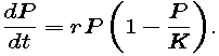
We may account for the growth rate declining to 0 by including in the model a factor of 1 - P/K -- which is close to 1 (i.e., has no effect) when P is much smaller than K, and which is close to 0 when P is close to K. The resulting model,

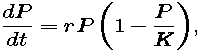
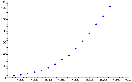
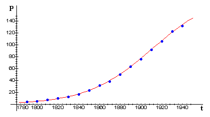
is called the logistic growth model or the Verhulst model. The word "logistic" has no particular meaning in this context, except that it is commonly accepted. The second name honors P. F. Verhulst, a Belgian mathematician who studied this idea in the 19th century. Using data from the first five U.S. censuses, he made a prediction in 1840 of the U.S. population in 1940 -- and was off by less than 1%.

This table shows the data available to Verhulst:

Date (Years AD)	Population (millions)
1790	3.929
1800	5.308
1810	7.240
1820	9.638
1830	12.866
1840	17.069

The following figure shows a plot of these data (blue points) together with a possible logistic curve fit (red) -- that is, the graph of a solution of the logistic growth model.

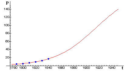
The next figure shows the same logistic curve together with the actual U.S. census data through 1940. This emphasizes the remarkable predictive ability of the model during an extended period of time in which the modest assumptions of the model were at least approximately true.

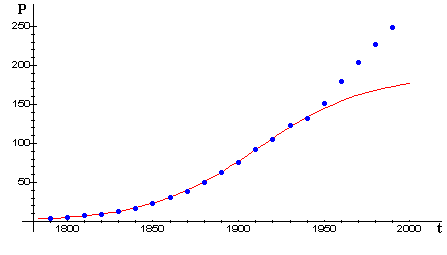
On the other hand, when we add census data from the most recent half-century (next figure), we see that the model loses its predictive ability. What (if anything) do you see in the data that might reflect significant events in U.S. history, such as the Civil War, the Great Depression, two World Wars?

For more on limited and unlimited growth models, visit the University of British Columbia. [Ed. Note: This link is not longer operable.]

1. The interactive figure below shows a direction field for the logistic differential equation

   

   as well as a graph of the slope function, f(P) = r P (1 - P/K). Click on the left-hand figure to generate solutions of the logistic equation for various starting populations P(0). [Note: The vertical coordinate of the point at which you click is considered to be P(0). The horizontal (time) coordinate is ignored.]

2. Explain why P(t) = 0 is a solution. A constant solution is called an equilibrium.
3. The logistic equation has another equilibrium, i.e., a solution of the form P(t) = constant. What is the constant? Explain how you know from the differential equation that this function is a solution.
4. If the starting population P(0) is greater than K, what can you say about the solution P(t)? What do you see in the differential equation that confirms this behavior?
5. If the starting population P(0) is less than than K, what can you say about the solution P(t)? What do you see in the differential equation that confirms this behavior?
6. Why is carrying capacity an appropriate name for K?

An equilibrium solution P = c is called stable if any solution P(t) that starts near P = c stays near it. The equilibrium P = c is called asymptotically stable if any solution P(t) that starts near P = c actually converges to it -- that is,

If an equilibrium is not stable, it is called unstable. This means there is at least one solution that starts near the equilibrium and runs away from it.

7. Is the equilibrium solution P = 0 stable or unstable? If stable, is it also asymptotically stable? Explain.
8. Is the equilibrium solution you found in step 3 stable or unstable? If stable, is it also asymptotically stable? Explain.

1. Which solutions of

   

   appear to have an inflection point? Express your conjecture in terms of starting values P(0). [For your convenience, the interactive figure from Part 3 is repeated here. Recall that the vertical coordinate of the point at which you click is P(0) and the horizontal coordinate is ignored.]

2. How is the location of the inflection point (when there is one) related to K? Record your conjecture -- you will check it in the next step.
3. Use your helper application to compute P"(t) in terms of P(t). (Don't forget the Chain Rule.) Use the resulting formula to confirm your preceding answers.
4. What is the significance of the inflection point in terms of population growth rate?

1. Separate the variables in the logistic differential equation
   

   Then integrate both sides of the resulting equation. (This is easy for the "t" side -- you may want to use your helper application for the "P" side.)

2. After calculating both integrals, set the results equal. If your helper application does not know about constants of integration, provide one in an appropriate place in your equation. Then solve the equation for P as a function of t.

3. Now use your helper application's differential equation solver to solve the logistic equation directly. If the resulting equation is not already solved for P as a function of t, use an additional "solve" step to complete the symbolic calculation.

4. The results from steps 2 and 3 are -- or should be -- formulas for the same family of functions. If the formulas do not look alike, reconcile any differences that you see. Show that one formula can be put in the form of the other. If the formulas have "arbitrary constants" in different places, show how the arbitrary constant in one formula is related to the arbitrary constant in the other formula.

5. In your integration in step 2, you may have encountered ln(P) and ln(K - P), both of which make sense if P is between 0 and K. But the second one does not make sense if P > K, so your formula may not be correct in this case. Change your equation in step 2 to one that would be correct if P > K, and solve again for P. Reconcile the result with the form generated by the differential equation solver in step 3, if possible. If you think the form generated by the DE solver does not work for P > K, explain why.

6. Suppose the starting population P(0) is a specific number P₀ (which may be either smaller or larger than K). Choose whichever solution form you prefer, and determine the value of the "arbitrary" constant (in terms of K and P₀) that produces a solution P(t) such that P(0) = P₀. Simplify as much as possible.

7. Explain why your solution function P(t) in step 6 approaches K as t becomes large.

8. For specific values of r, K, and P₀, plot the direction field and your solution function to verify visually that your formula is correct. Repeat with several combinations of the parameters, including values of P₀ both smaller and larger than K.

n the figure below, we repeat from Part 2 a plot of the actual U.S. census data through 1940, together with a fitted logistic curve. (Recall that the data after 1940 did not appear to be logistic.)

In this part we will determine directly from the differential equation

• how to tell whether a given set of data is reasonably logistic,

and, if so,

• what parameters r and K will give a good fit.

Our test case will be the U.S. Census data, first up to 1940, then up to 1990. In Part 6 we will study the same questions, but we will use the known form of the logistic solution from Part 4.

To determine whether a given set of data can be modeled by the logistic differential equation,

we have to estimate values of the derivative dP/dt from the data. We will do that by symmetric differences, as shown in the following figure. The slope dP/dt at a given census year t is approximated by the slope of the line joining the points 10 years earlier and 10 years later.

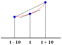
For example, the growth rate dP/dt in 1900 was approximately

[P(1910) - P(1890)] / 20.

Of course, for the period from 1790 through 1940, we can calculate these slope estimates only from 1800 through 1930, because we need a data point before and after each point at which we are estimating the slope.

We may rewrite the logistic equation in the form

In this form the equation says that the proportional growth rate (i.e., the ratio of dP/dt to P) is a linear function of P. Thus, we have a test of logistic behavior:

• Calculate the ratios of slopes to function values.
• Plot these ratios against the corresponding function values.
• If the resulting plot is approximately linear, then a logistic model is reasonable.

The same graphical test tells us how to estimate the parameters:

• Fit a line of the form y = mx + b to the plotted points. The slope m of the line must be -r/K and the vertical intercept b must be r.
• Take r to be b and K to be -r/m.

1. Use the commands in your helper application worksheet to construct symmetric difference estimates of dP/dt for the U.S. population data, to find ratios of dP/dt to the populations P, and to plot these ratios against P. You should find that the plot is roughly linear -- but only roughly.

2. Estimate the slope and vertical intercept of a line that will resonably fit the plotted points.

3. Check your work by plotting r (1 - P/K) on top of the plotted points. If necessary, adjust r and/or K until you are satisfied with the fit.

4. Interpret your final parameter values in terms of early growth of the U.S. population and ultimate size of the population. Are these numbers realistic? Why or why not?

5. Use the next set of commands in your worksheet to extend the logistic test to U.S. population data through 1990. In what way does the plot tell you that a logistic model for this data would not be reasonable?

In the preceding part, we determined the reasonableness of a logistic fit (up to 1940) and estimated the parameters r and K using only the differential equation, not the symbolic solution found in Part 5. Now we see what we can do by using the solution, which we recall has the form

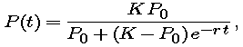
where P₀ is the population at whatever time we declare to be time 0. For example, if t = 0 in 1790, then P₀ = 3.929. For purposes of this exercise, we will make that choice of starting point and measure all times from 1790.

1. First, examine the solution with the parameters r and K from Part 6 by plotting the solution formula together with the data through 1940. (Don't worry if the fit is not very good -- we will see another way to estimate the parameters in the next two steps.)

In Part 5, as a step on the way to the symbolic solution, we saw that the solution would have to satisfy

ln P - ln (K - P) = r t + C,

that is, ln (P / (K - P)) should be a linear function of t with slope r. Thus, given a value of K, we can plot ln (P / (K - P)) against t and see if we get a straight line. (Note that there is no need to approximate rates of change for this type of test.) Since you already have an estimate of K from Part 6, it will not be a surprise if the plot looks pretty straight on the first try.

2. Use the commands in your worksheet to test the data for this type of fit. If your plot does not appear to be sufficiently straight, adjust K, recompute the data, and replot until you are satisfied that the plot is as straight as you can make it.

3. From the approximately linear relationship between
   ln (P / (K - P))

   and t in step 2, make a new estimate of r.

4. Replot your solution formula, along with the data, using your new value of r (and your new value of K if you changed it). If your plot is not yet satisfactory, repeat steps 2 and 3 until you are satisfied that you have the best values for K and r that you can get.

1. Explain in your own words the difference(s) between an exponential growth model and a logistic growth model.

2. The U.S. Census data from 1790 through 1940 was roughly logistic. What happened after that to interrupt this pattern?

3. Explain in your own words the meanings of the parameters r and K in the logistic differential equation

4. Sometimes the graph of the solution of a logistic equation has an inflection point. How is the location of this inflection point related to K? What is the significance of the inflection point in terms of population growth rate?

5. Suppose a population has a logistic growth rate and the starting population is greater than the carrying capacity. What would you predict about the future of the population? Why?

6. In our second attempt at fitting parameters to the U.S. population data (Part 7), we had the advantage of starting with a good estimate of K, the maximum supportable population -- but only because we did the fit in Part 6 first. Suppose you had only a plot of the data, as in the figure below. How would you estimate K from this plot? Would your estimate be close to the final value of K you chose in Part 7? Explain.