An Introduction to Population Ecology
The ability to predict the population size of a group of individuals is extremely useful to the study of ecology. It allows for the estimation of the various effects imposed upon a group by internal and external forces. We note that the word force has a different meaning in population modeling than in physics. You can think of these forces as factors that impact the population – for example, availability of food, spread of disease, interactions with other species. These forces can then be divided into density-independent forces and density-dependent forces.
Brandon Hale is a senior undergraduate at Murray State University. Maeve McCarthy is an Associate Professor of Mathematics at Murray State.
With no forces acting upon a population, we expect the population to have simple exponentially increasing growth (Vandermeer & Goldberg, 2004). Mathematically, we expect a population function whose rate of growth increases with the population’s size, that is,
![]()
This differential equation says that the rate of change in population size over time (dP/dt) increases by a proportional rate of growth (r) multiplied by the current population size (P). The biological force modeled here is an example of a density-independent force, because it depends only on the population P, not on external forces such as crowding or food supply.
We know from calculus that the solution of this equation is P(t) = P0ert. The graph of this exponential function (Figure 1) shows the behavior of the population over time. Biologists call this a J-shaped curve, and it is the foundation for all of the ecological models that we will discuss in this module (Molles, 2004; Vandermeer & Goldberg, 2004).

Figure 1. The exponential function has a J-shaped curve.
The exponential curve is best used for microorganisms, especially bacteria. Figure 2 shows the growth of a population of Escherichia coli bacteria. Notice that the population begins with just three bacteria, and the population has doubled within 20 minutes. Within three hours, the population has increased dramatically! (To see the figure in full size and resolution, click on the reduced figure shown here.)
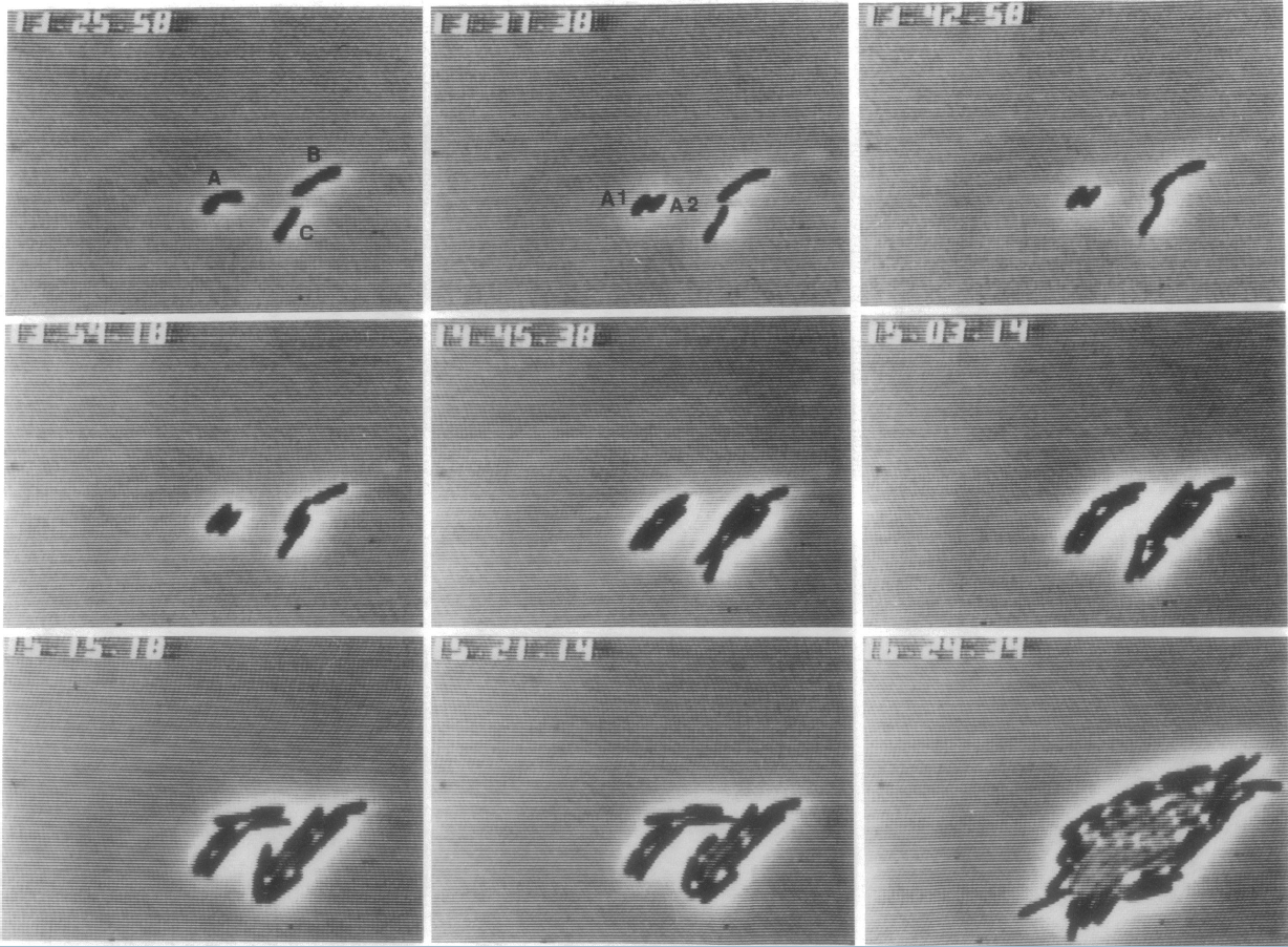
Figure 2. Formation of an Escherichia coli K-12 Microcolony from
three neighboring cells, by James Shapiro and Clara Hsu.
Source: American Society for Microbiology Microbe Library
Used by permission of James Shapiro.
We can use the doubling time to calculate the rate of growth for the E. coli population. If the initial population is P0, then the doubling time T for the population is the time required for the population to reach 2P0. This requires erT = 2. Solving for r, we find r = ln(2)/T. Since T = 20 minutes, we have r = 0.035 min-1.That means the bacteria population increases at a rate of approximately 3.5% per minute, which is equivalent to 816% per hour! This is an incredibly fast rate of increase.
For microbes, this may not be a problem. The entire colony of E. coli in the bottom right of Figure 2 could easily fit on the head of a pin. However, for larger organisms, exponential growth can be maintained for an extended length of time only under very rigid (and often unrealistic) conditions (Molles, 2004). For such organisms, logistic growth (next page) is more realistic.
Exercises
- If a population doubles every 5 hours, what is its rate of increase?
- If a population triples every 5 hours, what is its rate of increase?
- Suppose that the rate of increase for a particular bacterium is r = 0.24, how long does the bacterium take to double its population?
Published October, 2005
© 2005 by Brandon M. Hale and Maeve L. McCarthy
An Introduction to Population Ecology - Introduction to Population Modeling
The ability to predict the population size of a group of individuals is extremely useful to the study of ecology. It allows for the estimation of the various effects imposed upon a group by internal and external forces. We note that the word force has a different meaning in population modeling than in physics. You can think of these forces as factors that impact the population – for example, availability of food, spread of disease, interactions with other species. These forces can then be divided into density-independent forces and density-dependent forces.
Brandon Hale is a senior undergraduate at Murray State University. Maeve McCarthy is an Associate Professor of Mathematics at Murray State.
With no forces acting upon a population, we expect the population to have simple exponentially increasing growth (Vandermeer & Goldberg, 2004). Mathematically, we expect a population function whose rate of growth increases with the population’s size, that is,
![]()
This differential equation says that the rate of change in population size over time (dP/dt) increases by a proportional rate of growth (r) multiplied by the current population size (P). The biological force modeled here is an example of a density-independent force, because it depends only on the population P, not on external forces such as crowding or food supply.
We know from calculus that the solution of this equation is P(t) = P0ert. The graph of this exponential function (Figure 1) shows the behavior of the population over time. Biologists call this a J-shaped curve, and it is the foundation for all of the ecological models that we will discuss in this module (Molles, 2004; Vandermeer & Goldberg, 2004).
Figure 1. The exponential function has a J-shaped curve.
The exponential curve is best used for microorganisms, especially bacteria. Figure 2 shows the growth of a population of Escherichia coli bacteria. Notice that the population begins with just three bacteria, and the population has doubled within 20 minutes. Within three hours, the population has increased dramatically! (To see the figure in full size and resolution, click on the reduced figure shown here.)
Figure 2. Formation of an Escherichia coli K-12 Microcolony from
three neighboring cells, by James Shapiro and Clara Hsu.
Source: American Society for Microbiology Microbe Library
Used by permission of James Shapiro.
We can use the doubling time to calculate the rate of growth for the E. coli population. If the initial population is P0, then the doubling time T for the population is the time required for the population to reach 2P0. This requires erT = 2. Solving for r, we find r = ln(2)/T. Since T = 20 minutes, we have r = 0.035 min-1.That means the bacteria population increases at a rate of approximately 3.5% per minute, which is equivalent to 816% per hour! This is an incredibly fast rate of increase.
For microbes, this may not be a problem. The entire colony of E. coli in the bottom right of Figure 2 could easily fit on the head of a pin. However, for larger organisms, exponential growth can be maintained for an extended length of time only under very rigid (and often unrealistic) conditions (Molles, 2004). For such organisms, logistic growth (next page) is more realistic.
Exercises
- If a population doubles every 5 hours, what is its rate of increase?
- If a population triples every 5 hours, what is its rate of increase?
- Suppose that the rate of increase for a particular bacterium is r = 0.24, how long does the bacterium take to double its population?
Published October, 2005
© 2005 by Brandon M. Hale and Maeve L. McCarthy
An Introduction to Population Ecology - The Logistic Growth Equation
Exponential growth can be maintained for an extended length of time only under rigid conditions (Molles, 2004). The impact of the population on the environment generally increases as a limiting resource that the population relies on decreases.
Imagine a population of deer in the forest. They consume the various shrubbery and low leaves of trees. At first, while the population of deer is small, there is no problem with finding enough vegetation to sustain them. However, as the population continues to increase, the vegetation becomes more difficult to find. This creates density-dependence, which is one of the population’s intraspecific forces (Vandermeer & Goldberg, 2004). Other intraspecific forces include competition for mates, territory, or sunlight, as well as diseases or parasites. As a result, we have to modify the exponential growth equation to accommodate these density-dependent forces (Molles, 2004; Vandermeer & Goldberg, 2004).
Let’s suppose that the proportional rate of growth depends on the population density. Many populations in nature increase toward a stable level known as the carrying capacity, which we denote K. The carrying capacity of a population represents the absolute maximum number of individuals in the population, based on the amount of the limiting resource available. We can incorporate the density dependence of the growth rate by using r(1 - P/K) instead of r in our differential equation:
![]() .
.
In some textbooks this same equation is written in the equivalent form
![]()
This differential equation (in either form) is called the logistic growth model. Biologists typically refer to species that follow logistic growth as K-selected species (Molles, 2004).
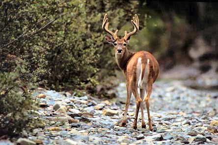
Figure 3. White-tailed deer.
Source: Deer Stock Photography © Steven Holt/stockpix.com
Used by permission from Stockpix.com
Example
Let’s consider the population of white-tailed deer (Odocoilus virginianus, shown in Figure 3) in the state of Kentucky. The Kentucky Department of Fish and Wildlife Resources (KDFWR) sets guidelines for hunting and fishing in the state, and it reported an estimate of 900,000 deer prior to the hunting season of 2004. Johnson (2003) notes: “A deer population that has plenty to eat and is not hunted by humans or other predators will double every three years.” This corresponds to a rate of increase r = ln(2)/3 = 0.2311. (This assumes -- with plentiful food supply and no predation -- that the population grows exponentially, which is reasonable, at least in the short term.) The KDFWR also reports deer densities for 32 counties in Kentucky, the average of which is approximately 27 deer per square mile. Suppose this is the deer density for the whole state (39,732 square miles). The carrying capacity K is 39,732 sq. mi. times 27 deer/sq. mi. or 1,072,764 deer.
 Let’s investigate the logistic growth model by using these values in the Ecological Models Maplet -- just click on the button at the right --you need to have Maple v9.0 (or higher) installed on your machine to run this program. The maplet should open in a new window and look like Figure 4.
 |
Figure 4. Opening Maplet Window |
Choose the radio button for the Logistic Model, and click the “OK” button. A new window will appear. You can use the maplet to see the logistic model’s behavior by entering values for the initial population (P0), carrying capacity (K), intrinsic rate of increase (r ), and a stop time. We’ve already entered some values, so click on “Graph”, which should produce Figure 5.
We’re using mathematical units rather than biological ones. For example, 25 time units could mean 25 years or 25 minutes, depending on the biological situation. For the case of deer in Kentucky, the time units are in years, and P and K are measured in thousands. Don’t be alarmed if you see 0.4 units for population -- in this case, that would mean 400 deer. However, you should be concerned if you see negative numbers for population!
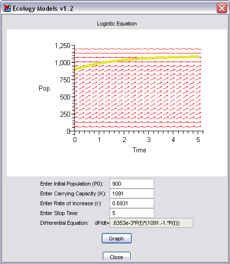
Figure 5. Maplet graph for the Logistic Model with Kentucky deer data.
Exercises
-
For the Kentucky deer population, P0 = 900,000 deer, K = 1,072,764 deer, r = 0.2311 per year. Describe the behavior of the population over 100 years. How does the behavior relate to the carrying capacity K?
-
Using the differential equation, find the stable equilibrium solutions. How do they relate to K?
-
Where is the graph steepest? What’s happening to the species at that time?
-
What do the red arrows represent?
-
Change the initial population P0 to 1.2 million deer, and graph the solution again. Explain what you see.
-
Change the initial population P0 to 500,000, and graph the solution again. Explain what you see.
-
Try using different values of K. What impact does this have on the population?
-
What if you increase the rate of increase r? What if you decrease it? Try some negative values of r. What happens to the species?
-
According to the KDFWR, Owen County, KY, had the highest population density of deer in the state in 2003 at 47 deer per square mile. Owen County is approximately 352.1 square miles. How many deer live in Owen County?
-
If 27 deer per square mile is optimal, what is the carrying capacity of Owen county? What does this tell you about the deer population?
-
Assume that the Kentucky rate of deer population increase (23.11% per year) also applies to Owen County. How many years will be required for the deer population to decrease to the Owen County carrying capacity?
An Introduction to Population Ecology - Harvesting a Population with Logistic Growth
![]()
If you closed your maplet window after the last set of exercises, you can start again with the button at the right. If your graphing window is still open, please close it now. Either way, from the main maplet window, choose the Logistic radio button, check the “Include Harvesting” checkbox, and click “OK”. A new window opens that includes a percentage harvesting rate, entered as a decimal fraction. For example, if 20% of the population is to be harvested each year, then h = 0.2. If there is to be no harvesting, set h = 0, and then the model reduces to the original logistic growth model.
Although the harvesting rate may be relatively small compared to the overall population, it can still have a large impact on the population. In combination with small intrinsic rates of increase typically seen in nature, it is easy to see why human actions (direct or indirect) have resulted in many endangered species (Edwards & Penney, 1999; Giordano et al., 2003).
Exercises
- For the Kentucky deer population without harvesting, P0 = 900,000 deer, K = 1,072,764 deer, r = 0.2311 per year. Try introducing some harvesting by changing the harvesting percentage to 5% or h = 0.05. What happens to the population over 10 years? Reduce the harvesting to 1%. What happens?
- What is the smallest percentage harvesting that you can have that will cause extinction with this species? You may need to increase the stop time so that you can see the long term trend. Give your answer in percentages to one decimal place.
- Using the harvesting percentage that you found in #2, increase the value of r. What happens? Find the smallest percentage harvesting that you can have that will cause extinction with this species. Repeat this a few times. What trend do you see? How would you explain it?
- In 2004, 124,752 deer were hunted and reported to the KDFWR, with previous years recording similar harvests. If the KDFWR targets at most 125,000 deer to be hunted every year, can the deer population be maintained?
- What is the maximum percentage hunting which the KDFWR can allow without the population decreasing below 500,000?
An Introduction to Population Ecology - The Explosion-Extinction Model

The Explosion-Extinction Model is best used for species that maintain themselves by fast reproductive rates. Molles (2004) describes such species as being r-selected. These species reproduce quickly and are generally regulated by an external force, such as predation or competition with another species, rather than by internal forces, such as density dependence. Such species are able to maintain their populations as long as their predators or competitors do not reduce the population below the minimum sustainable level.
A good example of an r-selected species is the oyster mussel (Epioblasma capsaeformis), shown in Figure 6. Mollusks reproduce rapidly by releasing hundreds of larvae, which are small and free-floating in the water, leaving them vulnerable to predation. The mollusk population will be maintained as long as enough larvae survive to grow, allowing the number of adults in the population to be maintained above the minimum sustainable level.

Figure 6. Oyster mussel (Epioblasma capsaeformis)
Source: Kentucky Department of Fish and Wildlife Resources
If an r-selected species is moved to an area where their predators are not found, the result can be dramatic. An introduced species often explodes (Figure 7, left), causing the indigenous species in the area to rapidly decline to extinction (Figure 7, right) as the two species compete for the same resource.

Figure 7. Population exploding (left) or dying out (right), depending on initial level
Exercises
If your graphing window is open, close it now -- or, if the maplet is not running, you can start it again with the button at the right. Choose the Explosion-Extinction radio button in the Main window.
- The default values are P0 = 12 units, M = 10 units, r = 0.03 per year and stop time = 100 years. Graph the population. Describe the behavior of the population over time.
- If the initial population is reduced to 10, will the population explode, go extinct, or neither? Change the initial population to 8. What happens?
- What do the red arrows represent? What kind of equilibrium is given by the value P = M? Describe what happens to the population when P0 > M; when P0 < M.
- If the rate of increase is reduced to 0.01 units per year and the initial population is 7 units, when will the population become extinct? What if r is increased to 0.2 units per year?
An Introduction to Population Ecology - Harvesting the Explosion-Extinction Model
![]() .
.
You can investigate the effect of this harvesting by returning to the main window, selecting both the Explosion-Extinction radio button and the Include Harvesting checkbox, and then clicking OK. (If the maplet is not running, use the button at the right to start it again.) If h = 0, everything works just like the normal Explosion-Extinction Model. Remember, h is the percentage of the population that is hunted or captured, expressed as a decimal fraction.
Exercises
- The default values are P0 = 20 units, M = 8 units, r = 0.04 per year and stop time = 100 years. Graph the population. What happens when you introduce a harvesting percentage of 7.5%?
- Try increasing the initial population. What happens? What is the smallest population that does not become extinct at this harvesting level? How would you summarize the effect of harvesting on the minimum sustainable level?
- Twenty individuals of an r-dependent species have been introduced into an area without its natural predators. The introduced species is known to increase rapidly at a rate of 40% per year, and it requires a population of only 8 individuals to maintain an increasing population. What percentage of the population must be hunted or captured in order to remove the introduced species?
An Introduction to Population Ecology - References
Edwards, H., & Penney, D. (1999). Differential Equations and Boundary Value Problems (2nd ed.). New Jersey: Prentice Hall.
Giordano, F. R., Weir, M. D., & Fox, W. P. (2003). A First Course in Mathematical Modeling (3rd ed.), pp. 395-402, 427-437. California: Brooks Cole.
Johnson, G. (2003). Exploding Deer Populations. Available online at http://www.txtwriter.com/onscience/Articles/deerpops.html (accessed 10/5/05)
Molles, M. C. (2004). Ecology: Concepts and Applications (3rd ed.), pp. 280-286, 347-371. New York: McGraw-Hill.
Vandermeer, J. H., & Goldberg, D. E. (2004). Population Ecology: First Principles, pp. 2-20, 178-195. New Jersey: Princeton University Press.