In 2010 the United States Census Bureau will once again conduct the decennial census. But apart from the interesting bits of information we will discover, such as the average number of bathrooms in an American home, why does the Bureau undertake this daunting task every ten years?

It’s because the United States Constitution requires it. In Article One, Section Two, the original text reads as follows:

Representatives and direct Taxes shall be apportioned among the several States which may be included within this Union, according to their respective Numbers, which shall be determined by adding to the whole Number of free Persons, including those bound to Service for a Term of Years, and excluding Indians not taxed, three fifths of all other Persons. The actual Enumeration shall be made within three Years after the first Meeting of the Congress of the United States, and within every subsequent Term of ten Years, in such Manner as they shall by Law direct. The Number of Representatives shall not exceed one for every thirty Thousand, but each State shall have at Least one Representative....

How we count the persons has thankfully changed since 1787. But the mandate of an “actual enumeration” remains. In fact, in the 1990s, the Census Bureau announced a plan to use statistical sampling to help achieve the required enumeration, rather than an actual headcount. After making its way through the courts, the Supreme Court ultimately ruled that sampling may not be used (see http://supct.law.cornell.edu/supct/html/98-404.ZO.html). But that is a topic for another day.

The Constitution requires an enumeration every ten years, as we read above, for the purpose of apportioning Representatives in the House of Representatives “according to their respective numbers.” Other than the specifications that each state must have a Representative, and that the number of Representatives shall not exceed one for every thirty thousand, the Constitution provides no guidelines as to how the Representatives shall be apportioned. This is where the fun begins.

The first census was to be taken in 1790, less than three years after the ratification of the Constitution. Once the numbers were in, the Congress had to decide how to use the data to apportion the Representatives. They also had to decide how many Representatives the House should have. In the spring of 1792 they passed a bill to apportion the House, using a method proposed by Alexander Hamilton and now known as Hamilton’s method.

Here is the procedure:

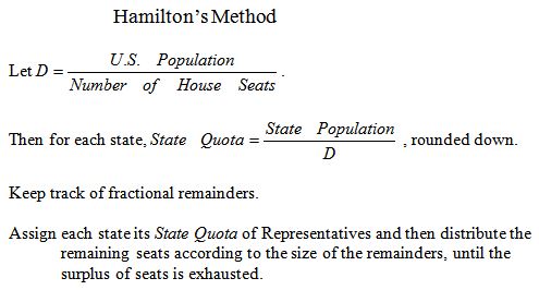
The divisor “D” in the method is the ratio of all U.S. residents to Representatives; it came out to a bit over 30,000 in this case. (Recall the Constitutional threshold above.) The State Quota is the number of seats each state is due, according to the divisor D. But while the apportionment must be in terms of whole numbers, these State Quotas are not. Therefore the method rounds the Quotas down, since rounding up could cause us to have more than the specified number of Representatives. But rounding down means we have apportioned fewer than the requisite number of seats. Hamilton proposes to allot the surplus seats, in order, to the states with the highest remainders after dividing by D. This process is followed until the given number of seats is assigned.

To see how this method apportioned the proposed 120 seats in the House, see the spreadsheet 1792 Hamilton.

Fair enough? Not necessarily. When the bill reached the desk of President Washington for his signature, there was a great division of opinion among his Cabinet members (one of whom was Alexander Hamilton, the Secretary of the Treasury). After listening to their opinions, Washington issued the first presidential veto in U.S. history. He objected that the bill unconstitutionally resulted in House members representing fewer than 30,000 persons, and that there was not a single divisor that could have resulted in the final apportionment. See http://avalon.law.yale.edu/18th_century/gwveto1.asp for the text of the President’s veto message to Congress.

Ten days after the veto, Congress passed a new method of apportionment, now known as Jefferson’s Method in honor of its creator, Thomas Jefferson.

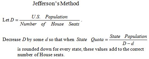
The “D” here is the same as it was for Hamilton. By decreasing D by some value d, Jefferson lowers the value of the denominator of the State Quota, thus raising the quota. Eventually the total of all State Quotas, rounded down, will match the predetermined number of House seats. The method therefore addresses one of Washington’s two objections: a single divisor will produce the apportionment.

To address the other concern, the Congress changed the number of House seats from 120 to 105. Thus a divisor of 33,000 was sufficient to produce the apportionment, and no state had a “persons to Representative” ratio of less than 30,000.

This method was approved by the President and was used to apportion the U.S. House from 1792 through 1842. But how different is it from Hamilton? If Hamilton’s method had been applied in 1792 to a House of size 105, 13 of the 15 states would have been assigned the same number of Representatives they received under Jefferson. It was Virginia that benefited under Jefferson (surprise!), while Delaware would have gained a seat under Hamilton that it instead lost to Virginia.

See the spreadsheet 1792 Jefferson for an illustration of the actual Jefferson apportionment of 1792 and a comparison with Hamilton.

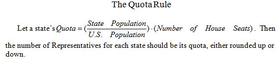
The fact that the affected states in the discrepancy just mentioned are Virginia and Delaware is no coincidence. In general, Jefferson’s method is biased in favor of larger states and against smaller ones. It violates what is called the “Quota Rule:

Here is a table that compares the populations and Representatives of Virginia and Delaware from 1790 through 1840:

By 1810, New York had overtaken Virginia as the most populous state in the Union. If we look at its numbers instead of Virginia’s, the discrepancy between that large state and Delaware is even more pronounced:

Using Jefferson’s method, New York always had its quota rounded up. On two occasions, its quota was rounded up more than one whole unit, in violation of the Quota Rule. In contrast, Delaware’s quota was rounded up only once. More striking are the cumulative results, showing New York well above and Delaware well below their expected totals.

There is a simple explanation for Jefferson’s bias toward the large states. The method works by lowering the divisor D by some d until the rounding fits the specified number of seats. But lowering the divisor causes the quotient to grow at a faster rate if the dividend is higher. For example,

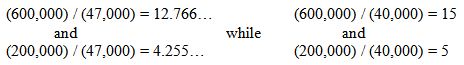
Lowering the divisor by 7,000 in each case raises the quotient by more than 2.2 in the case of the large dividend but only by 0.75 in the case of the small one.

As the decades wore on, the bias of Jefferson’s method in favor of the larger states was becoming more and more apparent. In 1822, in fact, Representative William Lowndes of South Carolina proposed an alternative procedure:

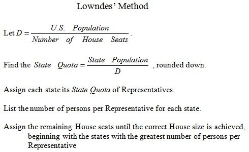
See the speadsheet 1822 Lowndes for an illustration of Lowndes’ method applied to the results of the 1820 census.

The method never had a real chance of gaining Congressional approval. As you may have seen in the file above, the method would have awarded the remaining 13 seats in the House to the smallest 13 states in the Union. The small states, of course, have very little voting power in the House as compared to the large ones. Jefferson’s method was retained.

The winds of change were blowing again in 1832. Former President John Quincy Adams, now a Representative from Massachusetts, proposed an inverse of Jefferson’s method:

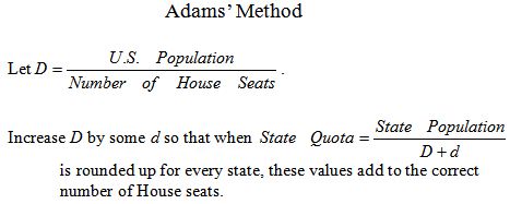
He proposed a House size of 250 and a divisor of 50,000 at the time. See the spreadsheet 1832 Adams for an illustration of the procedure. The file is set to a House size of 250, but ultimately the Congress passed a size of 240. If you save this or any other file linked to this article, you may play with the numbers yourself. In this case, the divisor may be adjusted until the rounded total of 240 is achieved.

If you experimented with the Adams file, you may have noticed the bias inherent in the method: it favors the smaller states at the expense of the large ones. We can see this by looking at a variant of the example that we had showing the bias in Jefferson’s method:

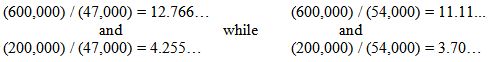
Increasing the divisor by 7,000 causes the larger quotient to decrease by about 1.65, while at the same time making the smaller quotient decrease by only about 0.5. The small states can let the large ones reduce their quotas at a faster rate until the predetermined number of House seats is achieved.

While Adams was pursuing this new procedure, Senator Daniel Webster, also of Massachusetts, received a proposal from James Dean, a professor of Astronomy and Mathematics at Dartmouth College.

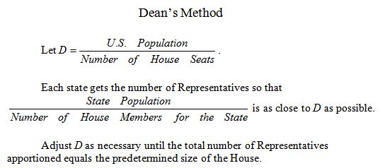
Although it may not appear this way at first glance, Dean’s method is equivalent to a method based on rounding. But in this case, the rounding is determined by the “harmonic mean:” the product of two numbers divided by their mean.

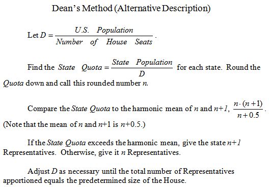
See the spreadsheet 1832 Dean for an illustration of this method. The file has two worksheets. The first shows just three states, New York, Maryland, and Louisiana. The left column is the potential number of Representatives for the state. The state’s population is divided by each potential number of Representatives, in turn, and compared to the given divisor (49,900 in this case). The number of Representatives assigned to that state is the number that minimizes the difference between the quotient and the divisor. The second worksheet illustrates the apportionment using the harmonic mean for all states. If you are interested in finding out more about the connection between Dean’s original description of the method and this rounding approach, download the Dean explanation.

Although its bias is not as strong as Adams’, Dean’s method does still tend to advantage the smaller states at the expense of the larger ones. Notice in the previous file that the large state of New York has its quota of 38.59 Representatives rounded down to 38 by Dean, while the small state of Louisiana had its quota of 3.46 rounded up to 4. As n increases in size, the harmonic mean increases toward n+0.5, so that for smaller states Dean allows a greater opportunity for rounding up than it does for the larger ones.

This proposal also appeared to have no chance of passage in the Congress, so Senator Webster proposed yet another alternative:

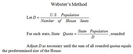
It is remarkable that it was not until the 1830s that a serious proposal had been put forth suggesting the use of ordinary rounding. And because it is based on ordinary rounding, Webster’s method is, unlike several of the others, unbiased. A state’s quota has just as much chance of having a remainder at or above 0.5 as it does having one below 0.5. See the spreadsheet 1832 Webster for an illustration of his method. As before, you may download the file and try different values of the divisor “D” until the correct total number of House seats is achieved.

Finally, Representative James K. Polk of Tennessee, later the 11th President of the United States, threw another idea into the mix: let’s just go back to using Jefferson’s method and use a divisor of 48,000. After he and others investigated many other possible divisors, it was discovered that using 47,700 instead of 48,000 would cause the quotas of the states of Kentucky, Georgia, and New York to advance past the next whole number, thus giving these three states an extra Representative each. From a political point of view, the fact that those three states collectively held about one-fourth of the House seats at the time sealed the deal: Jefferson survived the flurry of proposals in 1832 and was again used to apportion the House.

For a side by side tabular comparison of the four proposed apportionments of 1832 , see the spreadsheet 1832 Comparison.

The steadily-growing discomfort with Jefferson’s method reached a peak in 1842, after the numbers from the 1840 Census had been finalized. After noticing the advantage gained by Kentucky, Georgia, and New York when the divisor was changed from 48,000 to 47,700, a mad search for divisors began in the Congress. More than 30 different divisors were proposed in the House within the range from about 50,000 to 62,000. Cooler heads in the Senate prevailed, however. The Senate proposed the first (and only, with a brief exception) reduction in the size of the House in history. Not only that, it proposed scrapping Jefferson’s method in favor of that of Webster. The proposal passed.

Webster’s time was short-lived, however. In the 1850s it was Hamilton’s method, the one vetoed by Washington, that was adopted. In fairness to Webster, the two methods did agree on the 1852 apportionment. But it should also be mentioned that Hamilton’s method was never strictly followed, often because of the continuing entrance of new states into the Union.

The 1870s saw a new twist in the apportionment wars, one that spilled over into a Presidential election. In the apportionment of 1872, the House size was set to 292. Hamilton’s method was legally in place. Yet the actual apportionment approved by Congress differed in four states from the Hamilton apportionment. New York was assigned 33 seats in 1872, Illinois 19, New Hampshire 3, and Florida 2. But Hamilton’s method would have given New York 34, Illinois 20, New Hampshire 2, and Florida 1. Whatever Congress may have intended, the apportionment they approved is one that would have been given by Dean’s method for the Census of 1870.

Why is this such a big deal, outside of those four states? Because in the closely contested election of 1876, Samuel Tilden won the state of New York while his opponent, Benjamin Harrison, won the other three. Harrison beat Tilden in the Electoral College by a vote of 185 to 184. Had Hamilton’s method been followed, the count in the College would have been reversed and Tilden would have been elected! See the spreadsheet 1876 apportion for an illustration of the Hamilton calculation as compared to the actual apportionment and for a tabulation of the electoral votes in the election of 1876.

So in 1876, Hayes won under a Dean apportionment but would have lost under a Hamilton apportionment, even if no other factors had changed. Now let’s jump forward to the Presidential election of 2000. In the Electoral College, George W. Bush defeated Al Gore by a tally of 271 to 266. (Gore should have had 267 votes, but one of his electors from Washington, D.C. abstained.) Had the Congress used Jefferson’s method to apportion the House after the 1990 census, Gore would have garnered 271 electoral votes and become the President. Even more intriguingly, had Hamilton’s method been in place, the Electoral College vote would have been tied at 269 and the election thrown to the House of Representatives for resolution. Methods of apportionment do have practical consequences!

We must return now to the nineteenth century. Presidential elections were not the only place where some strange developments were occurring. In the 1880s the chief clerk of the Census Bureau computed the apportionment of the House for all sizes from 275 to 350. After all, if adjusting the divisor can produce “interesting” results, might not the same happen with an adjustment of the House size? The clerk’s computations revealed what is now known as the “Alabama Paradox”: for a House size of 299, Alabama would receive 8 Representatives, but if the House increased to 300, Alabama’s delegation would have dropped to 7. It would seem that any apportionment method exhibiting such undesirable behavior might be excluded from further consideration, although that is not the case. In fact, some today argue that Hamilton’s method is superior to all of the others, despite its paradoxical behavior.

See the spreadsheet Alabama paradox for an example of the effect using the census of 1870 and changing the House size from 270 to 280. In this illustration, it is Rhode Island which suffers the indignity of dropping from 2 Representatives in a 270 member House to 1 in a House of 280.

In the 1880s and 1890s, House sizes were chosen so that the calculations based on Hamilton’s method and Webster’s method would agree: 325 seats in the 1880s and 356 in the 1890s. But after the census of 1900, new “numbers games” surfaced.

Apportionments based on Hamilton’s method were calculated for all House sizes from 350 through 400. From sizes 382 through 391, Maine’s delegation switched from 3 to 4 seats and back again five different times. Colorado only suffered Maine’s plight once: it was to receive 3 seats for all values computed except for a House size of 357, in which case it would receive 2. The Chair of the House Select Committee on the 12th Census, no friend of the Colorado Populists, proposed a House size of 357. His proposal, alas, was defeated.

In fact, so was Hamilton’s method, once and for all. At least twenty years after the Alabama paradox had come to light, and after repeated observations of the numerical fluctuations that afflicted various states, Congress voted to replace Hamilton with Webster. The House size was set at 386, so that, of course, no state would lose a seat. It repeated itself ten years later when Webster was re-authorized with a House size of 433 (again, the smallest size so that no state loses a seat).

Before we move too fast into the twentieth century, let us return to 1907 and the entry of Oklahoma into the Union. Although Congress had adopted Webster, clerks for the Representatives, and others, examined what would have happened had Hamilton still been in place. They discovered yet another flaw in the method, known as the “New States Paradox.” In 1907 the House size was 386. According to its population at the time, upon entry into the Union Oklahoma was entitled to 5 Representatives, bringing the House size to 391. But when the Hamilton apportionment was re-calculated based on the new House size of 391, New York lost a seat to Maine! See the spreadsheet Hamilton new states paradox for an illustration of what happened. In brief, the new House size caused a shift in the remainders that Hamilton uses to apportion the surplus Representatives after all state quotas have been rounded down.

The 1920s saw the Congress move toward the apportionment method it still uses today. Joseph Hill of the Census Bureau proposed a new method. His goal was to keep the ratio of one state’s “people per Representative” to that of another as close to 1 as possible. In a nutshell, he said to choose the size of the House, and then assign seats to the states so that no transfer of a seat can reduce the percentage difference in representation between those states. Edward Huntington, a schoolmate of Hill’s, saw the new method, corrected an error in Hill’s calculations, and named the corrected procedure the Method of Equal Proportions. The method can be effected by assigning each state the number of Representatives such that the ratio of “people per Representative” to the ideal district size (the “D” below) is as close to 1 as possible.

This new method is equivalent to yet another method of rounding. In this case, though, the rounding is based on the geometric mean. The method is now commonly known as Hill’s Method, or the Huntington-Hill Method.

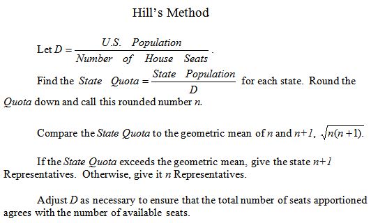
To see how Hill’s method is equivalent to this rounding procedure, download the Hill explanation.

The new method differed from the currently adopted Webster’s method in six states. Where they differed it was the larger states that suffered under Hill, not a good sign when passage of the method depends on a vote count in the House. In fact, for reasons we will not explore here, the Congress never re-apportioned seats in the 1920s, despite the Constitutional mandate to do so. Some in the Congress were so displeased with the state of affairs that a bill was introduced to enshrine a permanent apportionment method.

What finally passed in 1929 was a bill requiring the President to send to the Congress apportionments based on Webster, on Hill, and on the method used in the previous apportionment. If Congress took no specific action, the method last used would automatically be employed again. In the 1930s, not only was Webster the last used, but Webster and Hill agreed. This good fortune did not extend to the 1940s.

In 1941 the apportionments as computed by Webster and Hill differed in only two states. See the spreadsheet 1940 Webster vs. Hill. Webster gave 18 seats to Michigan and 6 to Arkansas, while Hill gave 7 to Arkansas and 17 to Michigan. It so happened that Michigan was a state that tended to be Republican while Arkansas was Democratic. A Representative from Arkansas sponsored a bill to use Hill’s method to apportion the House. Every Republican voted against the bill, while every Democrat (except those from Michigan) voted in favor. The bill passed and Hill’s method has been used to apportion the seats in a 435 member House ever since.

Differences exhibited between the Webster and Hill apportionments repeatedly appeared. While the two methods were identical after the 2000 Census, they produced different results in the 1940 through 1990 apportionments. Why should they differ?

Hill’s method tends to favor the smaller states at the expense of the larger ones, since its rounding is based on the geometric mean. The geometric mean is less than the ordinary (arithmetic) mean, and since the difference between these is greater for smaller quotas, Hill favors those smaller quotas. On the other hand, the geometric mean is closer to the ordinary mean than the harmonic mean is, so the bias of Hill is not as pronounced as the bias of Dean. See the spreadsheet 1980 - 2000 Webster v. Hill for an illustration comparing the Webster and Hill methods for the last three apportionments.

If you are interested you can find out more about two Supreme Court cases in the early 1990s. One upheld the validity of using Hill’s method to apportion the House, while the other allowed the Census Bureau to continue to count overseas military and civilian personnel and their families toward the populations of their home states. See http://www.law.cornell.edu/supct/html/91-860.ZO.html and http://www.law.cornell.edu/supct/html/91-1502.ZO.html for the texts of these decisions.

After the 2000 apportionment yet another case made its way to the Supreme Court. Utah saw a sizable gain in its population during the 1990s, yet did not increase its representation in the House after the 2000 Census. Advocates for the state examined the numbers and realized that if “imputed populations” (i.e., an estimate of the number of people living in a household after repeated failed attempts to get the actual number) were thrown out of the census, Hill’s method would shift a seat from North Carolina to Utah. The state brought suit to rule the use of imputed populations illegal, but the Supreme Court ultimately rejected this challenge. See http://www.law.cornell.edu/supct/html/01-714.ZO.html.

As we look ahead to 2010, we can use the U.S. Census Bureau’s 2007 population estimates, the most recently available as of this writing, to gauge what a newly re-apportioned House of Representatives may look like after the next census is completed. See the spreadsheet 2007 estimate for details. Both Hill’s and Webster’s methods are computed, although the two apportionments agree. Currently Texas stands as the only state poised to gain two seats in the House, while Arizona, Florida, Georgia, Nevada, and Utah would each gain a single seat. These gains are offset by the losses of single seats in Iowa, Louisiana, Massachusetts, Missouri, New York, Ohio, and Pennsylvania.

What is the future of the apportionment question? It is difficult to say. On the one hand, there has been no change in the apportionment method since 1941 and, other than a temporary adjustment when Alaska and Hawaii were added to the Union, there has been no change in the size of the House since the 1920s. On the other hand, Congress has the power to change either of these at any time. With each census there may be a discrepancy between the apportionments provided by different methods, prompting the disaffected parties to seek a remedy. And from an academic point of view, research continues to investigate the inherent biases, paradoxical behaviors, and other disadvantages of the various methods. In any case, the apportionment of Congress provides a unique blend of interesting mathematics and fascinating political maneuvering. Watch for the latest installment when the next decennial census is completed.

Balinski, Michel L. and Young, H. Peyton, Fair Representation: Meeting the Ideal of One Man, One Vote, 2nd edition, Brookings Institution Press, Washington, D.C., 2001.

Ernst, Lawrence R., Apportionment Methods for the House of Representatives and the Court Challenges, Management Science, Vol. 40, Issue 10 (1994), p. 1207-1227. Available at http://www.amstat.org/sections/SRMS/proceedings/papers/1992_118.pdf

Huntington, Edward V., The Mathematical Theory of the Apportionment of Representatives, Proceedings of the National Academy of Sciences, 1921 7:123-127. Available at PNAS: http://www.pnas.org/content/7/4/123.full.pdf+html

Neubauer, Michael G., and Zeitlin, Joel, Apportionment and the 2000 Election, The College Mathematics Journal, Vol. 34, No. 1, (2003), p. 2-10.

Toplak, Jurij, Equal Voting Weight of All: Finally 'One Person, One Vote' from Hawaii to Maine?, Social Science Research Network. Available at SSRN: http://ssrn.com/abstract=1001219