CalcPlot3D, an Exploration Environment for Multivariable Calculus
This dynamic Java applet developed with support from the NSF (Dynamic Visualization Tools for Multivariable Calculus, DUE-CCLI Grant #0736968)) allows the user to simultaneously plot multiple 3D surfaces, space curves, parametric surfaces, vector fields, contour plots, and more in a freely rotateable graph.
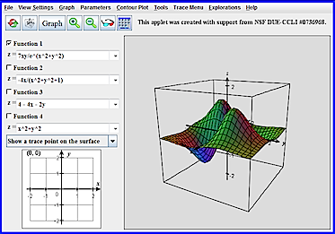 This tool is intended as a dynamic visualization and exploration environment for multivariable calculus. Use it to illustrate the geometric relationships of many of the concepts of multivariable calculus, including dot and cross products, velocity and acceleration vectors for motion in the plane and in space, the TNB-frame, the osculating circle and curvature, surfaces, contour plots and level surfaces, partial derivatives, gradient vectors and gradient fields, Lagrange multiplier optimization, double integrals as volume, defining the limits of integration for double and triple integrals, parametric surfaces, vector fields, line integrals, and more. See the corresponding web page for documentation and a list of guided explorations developed for students to use with this exploration applet.
INTENDED USES:
Instructors and students in multivariable calculus.
SOFTWARE SPECIFICATIONS:
Plugins: Java Plug-in (free) with any browser
Operating Systems: Mac, Windows, Linux, etc.
Open CalcPlot3D, an Exploration Environment for Multivariable Calculus in a new window
(Note: For the most up-to-date version of CalcPlot3D, see Paul's project website.)
CalcPlot3D, an Exploration Environment for Multivariable Calculus - Overview
This dynamic Java applet developed with support from the NSF (Dynamic Visualization Tools for Multivariable Calculus, DUE-CCLI Grant #0736968)) allows the user to simultaneously plot multiple 3D surfaces, space curves, parametric surfaces, vector fields, contour plots, and more in a freely rotateable graph.
This tool is intended as a dynamic visualization and exploration environment for multivariable calculus. Use it to illustrate the geometric relationships of many of the concepts of multivariable calculus, including dot and cross products, velocity and acceleration vectors for motion in the plane and in space, the TNB-frame, the osculating circle and curvature, surfaces, contour plots and level surfaces, partial derivatives, gradient vectors and gradient fields, Lagrange multiplier optimization, double integrals as volume, defining the limits of integration for double and triple integrals, parametric surfaces, vector fields, line integrals, and more. See the corresponding web page for documentation and a list of guided explorations developed for students to use with this exploration applet.
INTENDED USES:
Instructors and students in multivariable calculus.
SOFTWARE SPECIFICATIONS:
Plugins: Java Plug-in (free) with any browser
Operating Systems: Mac, Windows, Linux, etc.
Open CalcPlot3D, an Exploration Environment for Multivariable Calculus in a new window
(Note: For the most up-to-date version of CalcPlot3D, see Paul's project website.)
CalcPlot3D, an Exploration Environment for Multivariable Calculus - Using CalcPlot3D to Visually Verify Homework in Multivariable Calculus
One way to use CalcPlot3D, a versatile Java applet, is to demonstrate new concepts during multivariable calculus lectures. I often develop a new concept on the chalk board first and then take a couple minutes to make the concept come to life using the applet. Students find these demonstrations helpful and fun, and they bring variety to my presentations, helping students process the new concepts in a new way.
An even more exciting way to use CalcPlot3D in class is to engage in a visual exploration of new concepts using “What if…” types of questions. An example of a topic for which I find this approach works especially well is exploring the variety of possible parameterizations of a plane/space curve, paying special attention to the behavior of the velocity and acceleration vectors. Using these sorts of visual demonstrations in class improves student learning, but to fully engage students in the exploration and discovery process and give them the best chance of learning the geometric nature of the calculus concepts, I feel it is vital to give students opportunities to “play” with the concepts visually themselves. This article focuses on one way this can be done: by requiring students to visually verify solutions to particular homework problems and turn these in for a grade. [Another way this project supports student engagement and “play” is with the guided explorations being developed for various concepts. See the main project website to explore these. At this writing, there are explorations for Dot Products, Cross Products, Velocity & Acceleration Vectors, and Lagrange Multiplier Optimization.]
Below is a list of example topics where I often assign this type of visual verification exercise to my students to get them to begin using the applet on their own. Once they start using the applet in this way (because they have to), students often report using the applet more often on their own to explore additional exercises they complete from the textbook and on other assignments. Before giving a visual verification assignment involving new skills with the applet, I always demonstrate using CalcPlot3D to visually verify a similar problem we worked on the board. Once students have seen one example using the applet, most have little trouble completing the exercise on their own.
Without further discussion, let’s look at some examples of how this can be done! As you develop your own examples, please send them along to me! I would love to develop a library of useful ways to use this applet.
Examples
- Plane through Three Non-Collinear Points
- Line of Intersection of Two Planes
- Intersections of Other Types of Surfaces
- Contour Plots
- Level Surfaces
- Tangent Planes
- Directional Derivatives
- Taylor Polynomials of a Function of Two Variables (1st and 2nd degree)
- Lagrange Multiplier Optimization
- Riemann Sums of a Double Integral
CalcPlot3D, an Exploration Environment for Multivariable Calculus - Plane through Three Non-Collinear Points
An early topic that lends itself well to this sort of exercise is determining the plane determined by three  non-collinear points.
Exercise:
- Find the equation of the plane containing the points (2, 0, 1), (-1, 2, 3), and (0, 2, -2).
- Graph this plane along with the three points to verify that all threepoints lie on the plane. To do this, first solve the plane equation for z and graph the plane, entering it in Function 1. Then select Add a Point from the Graph menu, and enter the coordinates of one of the points. Select the default size and colors. (If you wish to vary these settings, be sure the points still show up well in the printout.) Repeat these steps to add the other two points. Rotate the plot to verify that the points lie on the plane and then find a clear view of the plane with the three points on it. Use the Print Graph menu option on the File menu at the top left corner of the applet to print out your resulting view and hand this printout in with this assignment.
Click here to open the CalcPlot3D applet in a new window.
Click here to open a pdf file which contains the instructions for the activity.
Answer: Plane equation is: z = (22 – 10x – 13y)/2
CalcPlot3D, an Exploration Environment for Multivariable Calculus - Line of Intersection of Two Planes
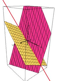 Visually verifying the line of intersection of two planes is another early topic where I get my students used to using the CalcPlot3D applet themselves. Below is an example of this type of problem:
Exercise:
- Determine the line of intersection of the following two planes. Write the parametric equations for this line, showing all work. \[ 2x + y - 2x = 5 \qquad \& \qquad 3x-6y-2z=15 \]
- Use the CalcPlot3D applet to display these two planes. To do this, solve each planar equation for z, and enter them in Functions 1 and 2 on the left side of the 3D plot window. Zoom out a couple times (if necessary) until you can see both planes along with their intersection. Now add the line of intersection. (To do this, choose Add a Space Curve from the Graph menu, and enter the parametric equations for the line.) Rotate the 3D view to verify that your line is indeed the intersection of the two planes. Rotate until you have a good view of the two planes and the line of intersection. Use the Print Graph menu option on the File menu at the top left corner of the applet to print out your resulting view and hand this printout in with this assignment.
Click here to open the CalcPlot3D applet in a new window.
Click here to open a pdf file which contains the instructions for the activity.
| Answer Line: | \(x = 3+14t\) | Here are the plane equations, solved for z: | |
| \(y=-1+2t\) | \(z=(2x+y-5)/2\) | ||
| \(z=15t\) | \(z=(3x-6y-15)/2\) |
CalcPlot3D, an Exploration Environment for Multivariable Calculus - Intersections of Other Types of Surfaces
See my paper on this topic online in the Proceedings of AMATYC 2010:
http://www.amatyc.org/Events/conferences/2010Boston/proceedings.html
It includes two examples of this type of problem along with steps to follow to visually verify the solutions using CalcPlot3D.
CalcPlot3D, an Exploration Environment for Multivariable Calculus - Contour Plots
Certain types of contour plots are not too difficult to create by hand. Many of these have contours that are lines, circles, or ellipses. But there are a lot of interesting functions whose contour plots are much more difficult to create by hand. I still require my students to be able to create contour plots of the first sort by hand, and they can certainly use the applet to visually verify their results. But I like to require them to use the applet to create contour plots for several functions whose contours are more complicated so they can improve their geometric intuition connecting the surface plots of various types of functions with their contour plots.
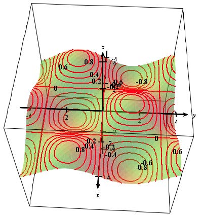
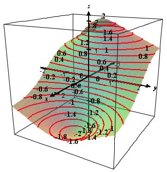
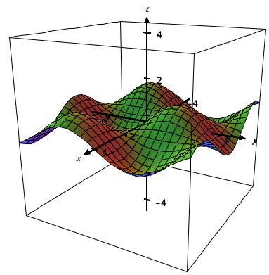
Exercise: Create contour plots for \(z = Cos(x)Sin(y)\) and \(z = -4x/(x^2+y^2+1) \). Print these contour plots and then for each one, click on the contour plot to see the contours as they appear on the surface. For each function, find a viewpoint that shows the surface and contours clearly and print this surface plot as well.
|
|
|
| \(z=Cos(x)Sin(y)\) | \(z=-4x/(x^2+y^2+1)\) |
*Sin(y)")
")
To create these contour plots, you will start by entering the function in Function 1 and graphing it. Then select the Draw Contour Plot option from the Contour Plot menu. A dialog will appear. Be sure that Function 1 is selected on the left. For the first function, you will then enter -1 for the First Step, 0.2 for the Step Size and 11 for the Number of Contours. Then click on the OK button to see the contour plot appear.
If you click on the contour plot, you will the 3D surface plot of the function will be graphed along with the contours on the surface.
For the second function, you will do the same thing, except you can enter -2 for the First Step, and 21 for the Number of Steps.
 |
 |
Click here to open the CalcPlot3D applet in a new window.
Click here to open a pdf file which contains the instructions for the activity.
CalcPlot3D, an Exploration Environment for Multivariable Calculus - Level Surfaces
It is difficult to draw many interesting level surfaces by hand, so I generally have my students use CalcPlot3D to do most of the work for this type of exercise. There are actually two ways to enter and graph the level surface equations for a particular function of three variables in CalcPlot3D:
- Solve each equation for z in terms of x, y, and C and enter the level surface using one or two functions of x and y, or
- Graph the level surface equation by Adding an Implicit Surface from the Graph menu and entering the equation for the level surface in the dialog box there.
If the surfaces are complicated enough, you may not have a choice. If you are not able to solve for z, you will need to use the Implicit Surface option.
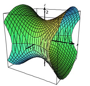
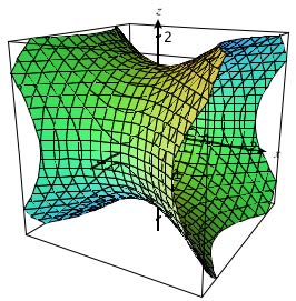
Here is an example I use in class shown both ways. \[ f(x,y,z) = z^2 - x^2 + y^2 \]
Setting \(f(x,y,z)=z^2-x^2+y^2=C\), we obtain the following equations if we solve for z.
 |
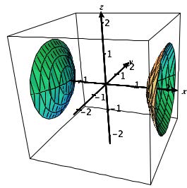 |
| C = 2 | C = -2 |
\(z=\sqrt{C+x^2-y^2}\)
\(z=-\sqrt{C+x^2-y^2}\)
For \(C=2\) we enter:
in Function 1, and in Function 2.
For \(C=-2\) we enter:
in Function 1, and in Function 2.
We can obtain the following graphs of these surfaces by graphing the implicit equations.
 |
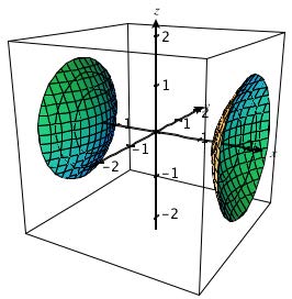 |
| \(z^2-x^2+y^2=2\) | \(z^2-x^2+y^2=-2\) |
\( z^2-x^2+y^2=2\) and \(z^2-x^2+y^2 = -2 \)
These equations will be entered as:
|
|
Click here to open the CalcPlot3D applet in a new window.
Click here to open a pdf file which contains the instructions for the activity.
CalcPlot3D, an Exploration Environment for Multivariable Calculus - Tangent Planes
I develop the equation of a tangent plane early in order to help students understand the geometric meaning of the total differential. In my opinion, it is not very satisfying to determine the tangent plane to a surface at a given point if you cannot visually verify the answer.
When I assign these exercises, I usually require students to submit a print-out from the applet showing their tangent plane, the surface and the point of tangency.
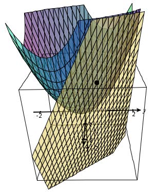
| Exercise: | Determine the tangent plane of the following surface at the point (1, 0.5) in its domain. Use CalcPlot3D to print the graph of this surface (with –2 to 2 on x- and y-axes) along with this tangent plane. Show the point of tangency. \[ z= f(x,y) = x^2 + xy + y^2 \] |
To create this plot, first enter the function in Function 1. Then enter the tangent plane function (solved for z) in Function 2. Graph these surfaces together. Then choose Add a Point from the Graph menu. Enter the coordinates of the point on the surface, and keep the default values for the other choices. To make it easier to see both surfaces, make them semi-transparent using either Ctrl-T or the Make Surfaces Transparent option on the View Settings menu.
Click here to open the CalcPlot3D applet in a new window.
Click here to open a pdf file which contains the instructions for the activity.
Answer: Tangent plane equation: \(z= 1.75 + 2.5(x - 1) + 2(y - 0.5)\)
CalcPlot3D, an Exploration Environment for Multivariable Calculus - Directional Derivatives
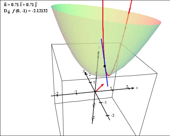 Exercise: Determine the directional derivative function for \( f(x, y) = x^2 + xy + y^2 + 1 \) in the direction of v = i + j. Then determine its value at the point (0, -1).
Use CalcPlot3D to graph this surface and show the appropriate tangent line on the surface at the point (0, -1) and displaying the unit direction vector and the correct directional derivative value.
To do this, first enter the function in Function 1. Then choose the directional derivative option from the drop-down menu just above the Trace Plot to the left of the 3D plot. You can then use the Trace Plot menu at the top of the applet to enter the point (0, -1) and the direction vector. I recommend hiding the edges (using the E key or the Hide Edges option on the View Settings menu) and also making the surface transparent
(using Ctrl-T or the Make Surfaces Transparent option on the View Settings menu). Rotate the plot until you can clearly see the direction vector, the surface, the tangent line, and the directional derivative value. Be sure it is the approximation of the exact value you obtained in your homework problem.
Click here to open the CalcPlot3D applet in a new window.
Click here to open a pdf file which contains the instructions for the activity.
CalcPlot3D, an Exploration Environment for Multivariable Calculus - Taylor Polynomials of a Function of Two Variables (1st and 2nd degree)
The way the Taylor polynomials of a function of one variable progressively converge to the graph of the function like y = cos x is really quite impressive and is inherently interesting. We can extend this topic into three dimensions using CalcPlot3D.
As an exercise, I require my students to generate the linear and quadratic Taylor polynomials of a function of two variables using the partial derivatives of the function evaluated at a particular point.
\( \begin{eqnarray} f(x,y) &\approx L(x,y) = f(a,b) &+ f_x(a,b)(x-a) + f_y(a,b)(y-b) \qquad (1^{st}\text{-deg. Taylor poly or tangent plane})\\ f(x,y) &\approx Q(x,y) = f(a,b) &+ f_x(a,b)(x-a) + f_y(a,b)(y-b) \\ &+\frac{f_{xx}(a,b)}{2}(x-a)^2 &+ f_{xy}(a,b)(x-a)(y-b) + \frac{f_{yy}(a,b)}{2}(y-b)^2 \qquad (2^{nd}\text{-deg. Taylor poly})\end{eqnarray}\)
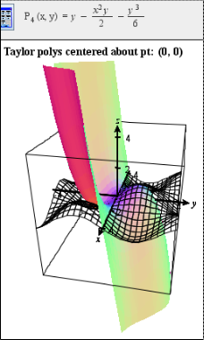
| Exercise: | Determine the 1st and 2nd degree Taylor polynomials in two variables for the given function. Simplify both polynomials. Show all work including all partial derivatives and using the formula clearly with functional notation in the first step. Please also provide a printout of the given surface along with each of the Taylor polynomials. (That’s 2 printouts all together.) Include the point on the surface where the polynomial is tangent to the surface. Use the Format Surfaces option on the View Settings menu so that the Taylor polynomial is reverse color and transparent so it’s possible to tell the two surfaces apart. If necessary, zoom out and the rotate to a view that shows the surfaces clearly. Then use the Print Graph option on the File menu of the applet to print the graph. \(f(x,y) = \sin(2x) + \cos y\) for x,y near (0,0) |
| Answers: | 1st-degree Taylor Polynomial of f: | 2nd-degree Taylor Polynomial of f: | |
| \(L(x,y)=1+2x\) | \(Q(x,y)=1+2x-\frac{1}{2}y^2\) | ||
 |
 |
There is also a feature of the applet that will allow you to demonstrate higher-degree Taylor polynomials for a function of two variables.
 Example:
- Graph the function, \(f(x,y)=\cos(x)\sin(y)\). Then zoom out to -4 to 4 in the x and y-directions.
- Now select the View Taylor Polynomials option from the Tools menu at the top of the applet. It will take a few seconds as the computer calculates the partial derivatives and creates the Taylor polynomials. This example is successfully calculated all the way up to the 15th degree polynomial. Once it is ready, the original function is graphed as a wireframe and the 1st degree Taylor polynomial (the tangent plane) is shown. A scrollbar appears along the bottom edge of the 3D plot. Use this scrollbar to scroll through the various Taylor polynomials of this function. Note that only odd degrees add new terms for this particular function. As you increase the degree of the Taylor polynomial notice how the polynomial of two variables fits the original surface better and better around the origin until it is a fairly good approximation of the whole visible surface at the 15th degree.
- To better view the Taylor polynomial itself (shown in the text window just above the 3D plot), you can click and drag on the equation and view all terms, dragging the equation left and right. You can also use the Tools menu option
 Use Factorials in Taylor Polynomials to switch this property on or off. Using factorials makes the form of the terms of the higher order Taylor polynomials easier to see, and the terms also generally take up less horizontal space each.
 - You can also vary the center point for the Taylor expansion using the Tools menu option just below View Taylor Polynomials. The default center point is the origin.
- Other nice functions to try centered about the origin include:
- \(f(x,y)=\cos(x)-\sin(y)\)
- \(f(x,y)=\sin(2x)-\cos(y)\)
- \(f(x,y)=\sin(x^2+y^2)\)
- \( f(x,y)=xe^y+1\)
- \(f(x,y)=e^{x^2+2x-y}\)
- \(f(x,y)=\arctan(xy)\)
- \(f(x,y)=\arctan(x+y)\)
Click here to open the CalcPlot3D applet in a new window.
Click here to open a pdf file which contains the instructions for the activity.
CalcPlot3D, an Exploration Environment for Multivariable Calculus - Lagrange Multiplier Optimization
 In multivariable calculus, we teach our students the method of Lagrange multipliers to solve constrained optimization problems. As we introduce this topic, many of us use some form of visual presentation to help students understand how we develop the Lagrange multiplier equation, i.e.,
\[ \nabla f(x,y) = \lambda \nabla g(x,y)\]
After demonstrating how this works in class with an example, I assign my students to print a visual verification of a homework problem showing both the contour plot with the constraint curve and the 3D surface plot with the constraint curve projected onto the surface showing the relative extrema visually.
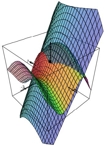
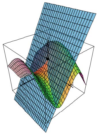
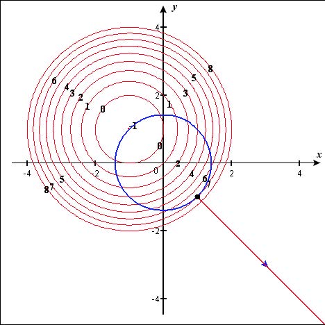
Exercise: Find the relative extrema of the function f subject to the given constraint, showing all work. Then graph the function in CalcPlot3D and create its contour plot with First Level: -1, Step size: 1, and number of contours: 10. Then add the constraint curve to the plot using the Add Constraint Curve option in the Display Contour Plot dialog. Use the scrollbar at the bottom of the contour plot to move the point to one of the relative extrema. Then print the contour plot. Finally click on the contour plot and print a view of the surface (along with the contours and the constraint curve projected on the surface) that makes it possible to see both extrema clearly.
\( f(x,y)=x^2+y^2+2x-2y+1\) Constraint: \(g(x,y)=x^2+y^2=2\)
 To obtain the images on the right using the applet:
- Enter x^2 + y^2 + 2x − 2y + 1 in Function 1. Zoom out once so the x and y values range from -4 to 4.
- To obtain the contour plot, choose the Draw Contour Plot option on the Contour Plot menu at the top of the applet.
- On the Display Contour Plot dialog, be sure Function 1 is selected, and enter First Level: -1, Step size: 1, and number of contours: 10.
- To display the constraint curve, select the second option on the Add Constraint Curve menu at the top of this Display Contour Plot dialog. This option is labeled, Circle centered at origin.
- Enter 2 as \(\mathbb{R}^2\) and click on the OK button.
- Now click on the OK button of the Display Contour Plot dialog and you should see the contour plot and the constraint curve appear.
- By default, the gradient vectors of f and g are displayed, \(\nabla f\) is red and \(\nabla g\) is blue. To watch them vary along the constraint curve, use the scrollbar located at the bottom of the 3D plot.
- We can visually verify that these gradient vectors are either parallel to each other or \(\nabla f=0\) when we obtain a relative extremum of f subject to the constraint, in both cases satisfying the Lagrange Multiplier equation.
- Now click on the contour plot in the large 3D plot window. The surface above will appear. Use the right arrow key to rotate the 3D graph to the right about the z-axis until you see a clear view of the relative extrema. Then use the scrollbar again to move along the trace of the constraint curve on the surface to verify the relative extrema we found earlier.
Click here to open the CalcPlot3D applet in a new window.
Click here to open a pdf file which contains the instructions for the activity.
CalcPlot3D, an Exploration Environment for Multivariable Calculus - Riemann Sums of a Double Integral
When introducing double integrals, I like to show the students how we can use rectangular prisms to approximate the volume of the solid region between the region of integration (in the xy-plane) and the surface. It is nice to connect these approximations to the value we obtain by evaluating the corresponding double integral. Here is an exercise students can do to improve their understanding of this connection.
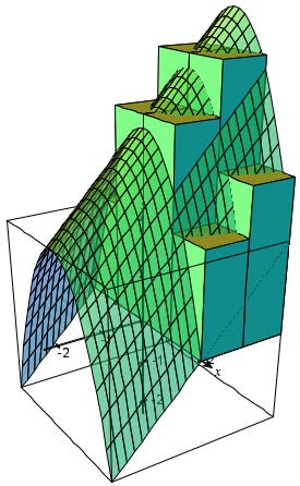
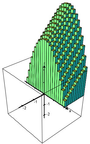
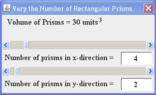
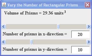
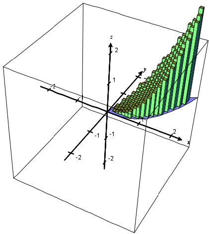
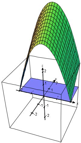 Exercise: Use 8 rectangular prisms to approximate the volume of the solid region between \(f(x,y)=4-x^2+y\) and the rectangular region R in the xy-plane given by \(-2\leq x \leq 2\) and \(0\leq x \leq 2\). Then use a double integral to find the exact volume of this solid region. Show all work on paper for both parts. Then use CalcPlot3D to create a graph of the region in the xy-plane along with the rectangular prisms you used and the surface above the region. Print a view of this graph that shows the surface and the rectangular prisms well. Use the Show grid scrollbars option on the Create Bounded Region dialog to vary the number of prisms in each direction. What do you notice happens to the volume of the prisms when you vary the number of prisms in the y-direction? Can you explain why this happens for this function? As you increase the number of prisms in the x-direction, does the volume of the prisms approach the exact volume you calculated? What is the volume of the prisms when there are 30 prisms in the x-direction?
 |
 |
 |
 |
To create these graphs:
- Graph the function \(z = 4 -x^2+y\).
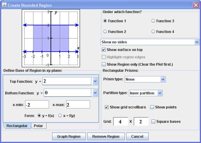
- Select Add a Region from the Graph menu.
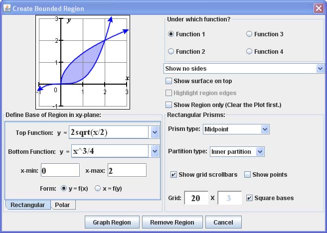
- The dialog shown at right will appear. Define the base of the region by entering \(y = 0\) for the bottom function and \(y = 2\) for the top function. Then enter -2 for x-min and 2 for x-max.
- At the top-right, Select the function number where you just graphed the function in step 1.
- Choose Show no sides from the drop-down menu just below the functions.
- Select to Show surface on top.
- Choose the Prism type to be Midpoint and then enter the number of prisms you want in the x- and y-directions next to the word Grid.
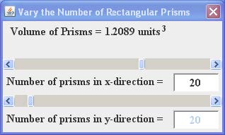
- Select Show grid scrollbars and then click on the Graph Region button.
- You can now use the scrollbars on the little dialog labeled Vary the Number of Rectangular Prisms to see what happens to the volume of the prisms as you vary their number in each direction. Note that the volume of the prisms is updated in this dialog as you do this.
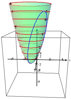
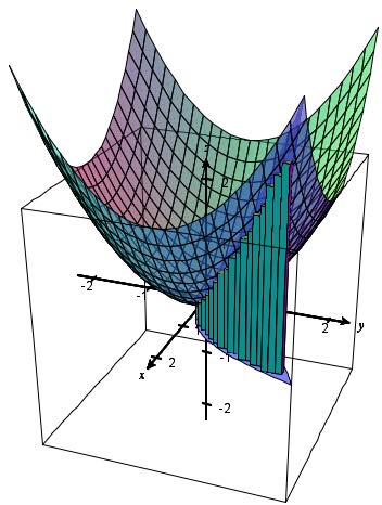
The graphs below show another example: \(f(x, y) = (x^2 + y^2)/2\) over the region in the xy-plane bounded by the graphs of \(y = \frac{x^3}{4}\) and \(y=2\sqrt{\frac{x}{2}}.\)
 |
 |
 |
 |
Click here to open the CalcPlot3D applet in a new window.
Click here to open a pdf file which contains the instructions for the activity.