Redistricting, a primer.

An excellent review of the redistricting process in the United States is A Citizen's Guide to Redistricting by Justin Levitt. [Levitt] In the United States a census is taken every 10 years. As population grows in one region and shrinks in another, states gain or lose seats in the House of Representatives. Additionally, as populations shift within states, some congressional districts have populations that are too large, others too small. As a result of these demographic shifts, states typically must redraw their congressional districts every decade. This process is called redistricting and must be completed before the first federal election following the release of the census data.

Redistricting Process: State governments are responsible for redrawing their congressional districts in response to changing census data. An ideal redistricting plan will generate districts of equal population that are contiguous and "compact". (We note here that the term compact does not refer to the mathematical concept of compactness, but rather to a qualitative notion of enclosing an area with a minimum of perimeter.) These three qualities are the most important. Secondary qualities include respect for city and county borders and respect for significant geographic features like rivers or mountain ranges. Tertiary qualities include having populations of similar interests, appropriate minority status, similar political affiliations.

The Constitution of the United States gives state legislatures the power to determine how each state's congressional representatives are chosen (Article 1, Section 4). Logically, this includes the power to draw the congressional districts that are each allocated a seat in the House of Representatives. Each state's legislature develops one or more preliminary redistricting plans, typically in a pre-existing legislative committee, or in a special committee formed for the sole purpose of redistricting. In some states, these special committees consist of citizens with no official ties to the state government, but most are made up of state representatives. [FairVote]

There is a large degree of variability in the methods used by these committees in the redistricting process. If a state has not experienced a large degree of demographic shift since the last census, for instance, its redistricting committee would probably use the state's current districts as a starting point for drawing the new ones. In states with shifting political leadership, a new majority party could also wish to drastically change the plan, in which case the legislative committee (presumably made up of majority party's members) might start with a more political map. [Levitt] Though these details vary greatly from state to state, almost all committees use some sort of software suite (Esri's ArcGIS or Caliper's Maptitude, for instance) to draw their plans. These plans are then subject to a vote by the whole of the state legislature, and often must also pass through the governor's office before they become official.

District Qualities: Our goal here is to present some of the technical issues associated with the task of redistricting. It should be noted that the process of redistricting is never likely to be wholly automated. That said, the people and committees in charge of developing redistricting plans still rely heavily on large data sets and computation to draw districts. We hope that by reading this paper and playing with our applet the reader will get an idea of what is involved and perhaps even contribute to the development of new tools to inform this process.

The quality of equal population has emerged over years of legal opinion to be the most important feature of any redistricting plan. Though it may seem obvious that all districts should have equal population to satisfy the "one person, one vote" philosophy, districts with large non-voting populations (e.g. children, non-citizens, people in prison) confer proportionally more weight to voters in those districts. [Bullock] There does not appear to be any inclination on the part of the courts to address this issue. Hence, we use the census data directly without having to remove ineligible voters.

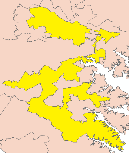
The quality of compactness of districts is less well-defined. There have been several measures of compactness used by the courts over the years. Generally, the area of a district should be enclosed by a boundary of minimum perimeter. For a given perimeter the circle encloses the most area. This follows from the famous isoperimetric inequality. [Oprea] Clearly, we cannot have circular congressional districts, but minimizing perimeter seems to be a desirable characteristic. However, courts have been willing to sacrifice compactness for the sake of other qualities—particularly in states under federal supervision via the Voting Rights Act. (reference) Consider, for example, the 12th district in North Carolina shown in this figure.

The 12th congressional district (yellow) of North Carolina in 2010. (arcGIS)

If a circle is considered the ideal compact shape, this district is far from compact. This figure shows a similarly non-compact district.

The 3rd congressional district (yellow) of Maryland in 2010. (arcGIS)

This figure shows the districts in Iowa.

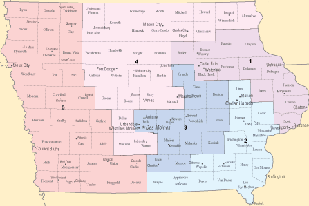
The congressional districts in Iowa in 2010. (from http://nationalatlas.gov)

Unlike the previous examples, these districts are relatively compact. Note also that this map respects county lines.

The work here focuses on the primary attributes of equal population, contiguity, and compactness. Given a population density function, \(\rho\), on a state, we present a few different ways of generating districts of equal population, that are compact and contiguous. We also include an applet that allows the user to draw their own district maps using a sweep circle algorithm.

The Population Density Function

All of the data collected by the United States during its decennial census is freely available from the Census Bureau. The data that we used throughout this paper comes from the 2010 data set. Our redistricting approach is driven primarily by the population density function, \(\rho\), of a particular state.

The Census Bureau provides population data down to the resolution of a single census tract. The Bureau also provides the geographic shapes of each census tract as they were during the collection of the data. If we let \(T\) be a census tract, \(A(T)\) be the area of the census tract (as projected upon the GCS North American 1983 [arcGIS]), and \(p(T)\) be the population of the tract, we define the population density function as \[\rho(\phi,\theta) = p(T)/A(T),\qquad (\phi,\theta)\in T\] The density function, \(\rho\), is a piecewise constant function defined within the boundaries of a single state. For definiteness, we assume that \(\phi\in [0,\pi]\) is latitude (with \(0\) at the North Pole) and \(\theta \in (-\pi,\pi]\) is longitude (with \(0\) at the Prime Meridian and \(\theta\) increasing to the east). Though not a sphere, we will assume a spherical approximation of the earth with radius \(R=3958.755\) miles [Moritz].

To facilitate numerical algorithms, we further discretize \(\rho\) using a uniform grid in the latitude/longitude domain as in the figure below. For simplicity, we assume that the state that we are redistricting is bounded by a spherical patch (some rectangle in the \((\phi,\theta)\)-plane) that is completely contained in both the northern hemisphere and in the western hemisphere. Hence, the latitudes spanning the state are contained in the interval \([\phi_{\min},\phi_{\max}] \subset [0,\pi/2]\) and the longitudes are contained in the interval \([\theta_{\min},\theta_{\max}] \subset (-\pi, 0]\). I.e. \(\phi_{\min}\) is the northern most latitude of the state and \(\theta_{\min}\) is the western most longitude of the state.

We discretize the spherical patch as \begin{eqnarray*} \phi_i & = & \phi_{\min} + \frac{\phi_{\max}-\phi_{\min}}{M},~i=0,1,\ldots M \\ \theta_j & = & \theta_{\min} + \frac{\theta_{\max}-\theta_{\min}}{N},~j=0,1,\ldots N. \end{eqnarray*}

A uniform latitude/longitude grid on the surface of a sphere

We then generate a discrete density function on the patch \(\rho_{ij} = \rho(x_i,y_j).\)

In order to reconstitute the population of a particular region, it is necessary to know the area of of each grid square in the discretization. Recall that each grid square of latitude and longitude represents a small patch on the surface of the earth. Furthermore, though the grid squares are uniform in the latitude and longitude domain, the actual surface area represented by each square depends upon its latitude again see this figure and this figure. We approximate the area of the patch with upper-left hand corner at \((x_i, y_j)\) by assuming that the earth is a sphere and using a spherical surface integral.

A flat projection of a uniform latitude longitude grid

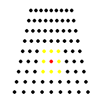
For later reference, the colored dots indicate a Moore-type neighborhood set. The red dot is the center of the neighborhood. The yellow dots are the neighbors of the center dot. Every dot is the center of an associated Moore neighborhood.

First we convert \((x_i,y_j)\) to spherical coordinates. \begin{eqnarray*} \phi_i & = & (90^\circ - x_i)\cdot \frac{\pi}{180^\circ} \\ \theta_j & = & y_j \cdot \frac{\pi}{180^\circ}. \end{eqnarray*} Then, \begin{eqnarray*} A(x_i,y_j) & = & \int_{\theta_j}^{\theta_{j+1}} \int_{\phi_i}^{\phi_{i+1}} R^2 \sin\phi \, d\phi d\theta\\ & = & R^2(\theta_{j+1} - \theta_j) (\cos(\phi_{i+1}) - \cos(\phi_i)). \end{eqnarray*} It follows immediately that the population of a particular grid square is well-approximated by \(\rho_{ij} A(x_i,y_j)\).

Sweepline Redistricting

The redistricting schemes we consider throughout this article are primarily concerned with equal populations and compact districts. For definiteness, consider the state of Washington with 9 legislative districts–the number of districts it had just prior to the 2010 census. Washington currently has 10 congressional districts, but 9 factors nicely and hence provides a better illustration of the concept. It is clear that there are a number of different ways to partition the state into regions with equal population. This paper will discuss two methods each of which can be adapted to provide a multitude of equal partitions.

In this section, we borrow a term from the mathematical literature of Voronoi tessellations [Okabe]. Some methods of generating Voronoi tessellations rely on an imaginary line that sweeps from left to right across a plane. When the line meets certain conditions, geometric events are generated that ultimately lead to a Voronoi diagram [Fortune].

Our first equal partitioning scheme borrows from this idea. We start with an imaginary vertical sweepline at the left most edge of the state of Washington. We sweep from left to right across the state. When the line has swept out a certain portion of the population, it leaves a copy of itself there marking the boundary of a region and continues on to sweep out the next region.

In an effort to draw 9 equal population districts as in this figure, a vertical sweepline first divides the state into three equal population regions. Subsequently, in each of the three regions, a horizontal sweepline divides the region into three equal population subregions. The result is 9 rectangular regions of equal population.

A sweepline redistricting of Washington state. Each of the 9 regions has equal population.

Notice in the figure that the second vertical partition is quite narrow. This results from the fact that it contains the densely populated Seattle-Tacoma area. While having equal population, these districts are not compact. They tend to be long and skinny instead of stout and blocky.

To emphasize the non-uniqueness of such partitions, imagine starting first with a horizontal sweepline and then generating subregions using vertical sweeplines. There would be 9 equal population districts, but they would be different from those pictured here.

How do we generate districts of equal population that are also compact? We move to another idea from the literature of Voronoi tessellations--that of sweepcircles.

Sweepcircle Redistricting

To improve the compactness of the regions in equal population partitions, we start with the most compact geometric shape-the circle. In this scheme, now considering Washington state with its current 10 congressional districts, we start with a manually placed set of 10 points within the state that will serve as the centers of 10 sweepcircles expanding at the same rate as in this figure.

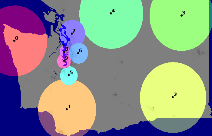
Redistricting with expanding sweepcircles.

The sweepcircles are allowed to expand until they encompass their share of the total population—in this case 1/10 of the total population. When a sweepcircle reaches this threshold, it ceases to expand while the remaining sweepcircles continue to expand. Notice in this figure that the circles in the Seattle area, 5, 6, 7, 8, and 9, have already halted because they have reached their population quota. This algorithm derives from a similar algorithm for computing Voronoi tessellations based on sweep circles. [Schueller]

In that algorithm, grid points at the boundary of the expanding sweepcircle "claim" neighboring open grid points. When a grid point encounters a grid point that has been claimed by another sweepcircle, a simple tie breaker is invoked and the disputed grid point is assigned to the region with the closer center.

In general, the resulting partition fails to generate a good set of districts. Still expanding circles wrap around halted circles often forming non-compact districts (though of equal population). Fortunately, the failed partition can often be used to inform us how to adjust the starting centers to generate a better set of districts. The reader can experiment with the iterative process of drawing districts based on sweepcircles using this applet.

The direct application of the results in Schueller to this problem is complicated by the fact that the computations occur on the surface of a sphere instead of on a flat plane. In the remainder of this section, we discuss, in the context of Schueller, how to address this complication.

Recall that the population density function is defined on a discrete mesh of points that is uniform in latitude and longitude. However, the distances between points in that mesh are not uniform as they lie on the surface of the earth (see figure).

The sweepcircle algorithm addresses the issue of generating expanding circles on rectangular grids as in this figure. In particular, it outlines a method of analyzing neighborhood sets around grid points to grow circular regions on discrete rectangular grids. The rate at which the sweep circle grows must be controlled in such a scheme or the circular geometry will be lost. This method allows the expanding regions to respond to and yield when other expanding regions are encountered.

Sweepcircle progression on a uniform, rectangular mesh using Neumann neighborhoods
(only north, south, east, west gridpoints).

The algorithm we employ in the applet uses Moore neighborhoods (see the red and yellow points in this figure). The Moore neighborhood of a grid point is made up of the 8 surrounding grid points. Compare this, for example, to the Neumann neighborhood where only the north, south, east, and west grid points are considered neighbors of the center point. The choice of neighborhood set affects the rate at which the sweepcircles can expand.

Haversine Distance. The notion of distance is important to the sweepcircle algorithm. In contrast to flat space, this mesh lies on the surface of the earth that we approximate by a sphere. The distance between two points on the surface of a sphere, if one is restricted to the surface of the sphere, is given by the length of the segment of the great circle that lies between the two points. Consider two such points in spherical coordinates \({\bf p}_1 = (R,\phi_1,\theta_1)\) and \({\bf p}_2 = (R,\phi_2,\theta_2)\). This distance is given by the Haversine distance function [Sinnott] \[d({\bf p}_1, {\bf p}_2) = 2R \arcsin \left( \sqrt{\sin^2 \left( \frac{\phi_2-\phi_1}{2} \right) + \cos(\phi_1) \cos(\phi_2) \sin^2 \left( \frac{\theta_2 - \theta_1}{2} \right) } \right).\]

To apply the algorithm, we must determine the initial radius of the sweep circle, \(r_0\), and the radial increment of the sweep circle at each step, \(\Delta r\). The initial radius is the smallest circumscribing circle of the Moore neighborhood set. The radial increment is the largest inscribed circle in the Moore neighborhood set. A typical Moore neighborhood in the discretization of a spherical patch in the northern hemisphere is shown in this figure.

A Moore neighborhood projection stretched according to the Haversine distance function. Line segments of like color represent like Haversine distances.

Radial Increment. Choosing a \(\Delta r\) that is too small will not affect the algorithm, so we find an inscribed circle for a neighborhood along the northernmost latitude where the neighborhoods are smallest. Such a \(\Delta r\) will then be appropriate for all of the neighborhoods in the grid.

Assuming a Moore neighborhood, to find the inner radius of a northernmost neighborhood, we need to find the minimum Haversine distances between neighbors shown in light blue (horizontal) and those shown in green (vertical) in the figure. A circle whose radius is the minimum of these distances will be inscribed like the red, dashed circle in the figure.

Referring to the discretization used for the population density function, we assume a mesh size in the longitudinal direction \[h=\frac{\theta_{\max}-\theta_{\min}}{N}\] and in the latitudinal direction \[k=\frac{\phi_{\max}-\phi_{\min}}{M},\] we compute these distances.

The vertical distances (green) are the same and, with respect to the Haversine function, are characterized by having endpoints with equal longitudes, say \(\theta_i\). The distance function is simplified by this observation and is given by \[ 2R \arcsin \left( \left|\sin\left( \frac{k}{2} \right)\right| \right).\] For small, positive \(k\), this simplifies to \(Rk\).

As noted, we are only concerned with distances along the top edge of the neighborhood set because, for grids in the northern hemisphere, the top edge distances are the shortest horizontal distances. The horizontal distances along the top edge are the same and are characterized by having endpoints with equal latitude, \(\phi_{\min}\). This again simplifies the distance function and the distances are given by \[2R \arcsin \left( \left|\cos(\phi_{\min}) \sin \left( \frac{h}{2} \right) \right| \right).\]

Hence, a radial increment that will enable the sweep circle algorithm to work correctly is \[\Delta r = R \min\left\{k, 2\arcsin \left( \left|\cos(\phi_{\min}) \sin \left( \frac{h}{2} \right) \right| \right) \right\}.\]

Since the patch is in the northern hemisphere, we can drop the absolute values to get \[\Delta r = R \min\left\{k, 2\arcsin \left[ \cos(\phi_{\min}) \sin (h/2)\right] \right\}.\]

Initial Radius. Similarly, choosing an \(r_0\) that is too large will not adversely affect the sweepcircle algorithm, so we find a circumscribing circle for a neighborhood along the southernmost latitude where the neighborhoods are largest. Such an \(r_0\) will then be appropriate for all of the neighborhoods in the grid.

We will find the maximum of the diagonal Haversine distances shown in dark blue and purple in this figure for a neighborhood at the southernmost boundary of the patch. Since our patch is in the northern hemisphere, it is clear that the lower diagonals are the longest (and have the same length) hence it suffices to compute the length of one of these diagonals. Supposing that we consider the neighborhood with its lower right corner at \((\phi_{\max},\theta_{\max})\), the length of this diagonal and hence the radius of a circumscribing circle is \[r_0=2R \arcsin \left( \sqrt{\sin^2 \left( \frac{k}{2} \right) + \cos(\phi_{\max}) \cos(\phi_{\max}-k) \sin^2 \left( \frac{h}{2} \right) } \right).\]

The Redistricting Applet. The applet included in this paper is written in the Processing programming environment. It is able to run in Javascript enabled browsers via the Processing.js library. The algorithm used to draw the expanding circles is based on sweepcircles with parameters computed according to the formulas derived in this section.

The user is invited to place the centers of the sweepcircles and to execute the algorithm. There are 10 centers corresponding to the 10 congressional districts that Washington currently claims. A score is generated that attempts to rate the quality of your districting plan. The score is a combination of how much unclaimed population remains at the conclusion of the algorithm and how compact the regions are. The user, informed by the current districting scheme and the score, is then allowed to move each of the 10 centers and re-execute the sweepcircle algorithm in hopes of improving the districts and the score.

Redistricting With SweepCircles

Algorithm written by Albert Schueller and Evan Kleiner

INSTRUCTIONS:

This is a map of the state of Washington with a light grey scale population density function overlayed. As the grey scale indicates, significant populations are concentrated around the Puget Sound area (Seattle) and near the middle of the eastern border (Spokane).

Your job is to create a set of congressional districts for the state. Begin by placing 10 points on the map with your mouse. These are the 'centers' of Washington's congressional districts. Once this is completed, the algorithm will begin and concentric circles will grow out of each center until they either reach their appropriate population (1/10 of Washington's total population), or until they are blocked off from further growth by the districts surrounding them. A table below the map will display the district populations as the algorithm runs. After all of the circles have stopped growing,your effort will be scored. (see Scoring)

You will then have the opportunity to move the centers so as to generate better districts than your previous attempt. This process repeats itself until you are satisfied with the districts you have generated. Please watch our tutorial video to see how it works. Good Luck!

Here we discuss two possible avenues of extending this work. The first comes from the literature of centroidal Voronoi diagrams. The second from the idea of crowd-sourcing.

Lloyd-type Iterations

The approach of the applet to finding an "optimal" redistricting plan is reminiscent of another algorithm related to Voronoi diagrams–that of the Lloyd algorithm for computing centroidal Voronoi diagrams. [Du] In a Lloyd algorithm, we start with a Voronoi diagram.

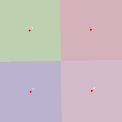
A Voronoi diagram for 4 centers (white) and the corresponding centroids (red).

A Voronoi diagram (VD) for a collection of points, called centers, is simply a partition of the set into regions where each point in the region is closer to its center than any other center. In general, the centroids of each region will not coincide with the centers of the regions.

The Lloyd algorithm moves the centers (white) to their corresponding centroids (red) and recomputes the Voronoi diagram and repeats. After many iterations, the centers and the centroids coincide and the result is known as a centroidal Voronoi diagram (CVD). Typically a CVD has a more regular appearance than an arbitrary VD.

A centroidal Voronoi diagram for 4 points (white) and the corresponding centroids (red).
Here they coincide after Lloyd iteration.

An interesting avenue of future exploration would be to develop a Lloyd-type algorithm for the redistricting applet. Rather than have the user manually move the centers to some new positions that may improve the redistricting plan, one could devise a systematic placement scheme that iteratively "improves" the districts. Perhaps, it adjusts to minimize perimeter. Or, more generally, perhaps the scheme adjusts to optimize a weighted list of other desirable characteristics that we have not addressed here.

Crowd-sourced Redistricting

Consistent with the interactivity of our redistricting applet, the authors can envision a scheme where the residents of a state are invited to play a redistricting game. The results of hundreds (or thousands) of players could be aggregated to build a starting point for state redistricting committees. This approach has the advantage of being more participatory and hence confers the democratic credibility that is so necessary to the redistricting process.

References

1. Bullock, Charles. Redistricting : the most political activity in America. Lanham, Md: Rowman & Littlefield, 2010
2. Du, Qiang, Vance Faber, and Max Gunzburger. "Centroidal Voronoi Tessellations: Applications and Algorithms." SIAM Review 41.4 (1999): 637.
3. Fortune, Steven. "A Sweepline Algorithm for Voronoi Diagrams." Algorithmica 2.1-4 (1987): 153-74.
4. "State By State Analysis." FairVote. N.p., 2000. Web. 18 July 2012.
5. Levitt, Justin. A Citizen's Guide to Redistricting. New York: Brennan Center For Justice, 2010. Brennan Center For Justice. Web. 11 July 2012. .
6. Moritz, H. (1980). Geodetic Reference System 1980, by resolution of the XVII General Assembly of the IUGG in Canberra.
7. Okabe, Atsuyuki, Barry Boots, Kokichi Sugihara, and Sung Nok. Chiu. Spatial Tessellations: Concepts and Algorithms of Voronoi Diagrams. Chichester [etc.: J. Wiley & Sons], 2000.
8. Oprea, John. Differential Geometry and Its Applications. Washington, D.C.: Mathematical Association of America, 2007.
9. Schueller, A. "A Nearest Neighbor Sweep Circle Algorithm for Computing Discrete Voronoi Tessellations." Journal of Mathematical Analysis and Applications 336.2 (2007): 1018-025.
10. Sinnott, R.W. "Virtues of the Haversine." Sky and Telescope 68.2 (1984): 159.

Acknowledgments

• The work here was completed under a Perry Summer Research grant from Whitman College. We are grateful to the donors that support this important program without which this work would not have been possible.
• We would also like to thank Amy Molitor, Adjunct Assistant Professor of Environmental Studies, for her invaluable help in obtaining population and map data from the ArcGIS software package.