- About MAA
- Membership
- MAA Publications
- Periodicals
- Blogs
- MAA Book Series
- MAA Press (an imprint of the AMS)
- MAA Notes
- MAA Reviews
- Mathematical Communication
- Information for Libraries
- Author Resources
- Advertise with MAA
- Meetings
- Competitions
- Programs
- Communities
- MAA Sections
- SIGMAA
- MAA Connect
- Students
- MAA Awards
- Awards Booklets
- Writing Awards
- Teaching Awards
- Service Awards
- Research Awards
- Lecture Awards
- Putnam Competition Individual and Team Winners
- D. E. Shaw Group AMC 8 Awards & Certificates
- Maryam Mirzakhani AMC 10 A Awards & Certificates
- Two Sigma AMC 10 B Awards & Certificates
- Jane Street AMC 12 A Awards & Certificates
- Akamai AMC 12 B Awards & Certificates
- High School Teachers
- News
You are here
Visualizing Lie Subalgebras using Root and Weight Diagrams
2.3 Weights and Weight Diagrams
An algebra \(g\) can also be represented using a collection of \(d \times d\) matrices, with \(d\) unrelated to the dimension of \(g\). The matrices corresponding to the basis \(h_1, \cdots, h_l\) of the Cartan subalgebra can be simultaneously diagonalized, providing \(d\) eigenvectors. Then, a list \(w^m\) of \(l\) eigenvalues, called a weight, is associated with each eigenvector. Thus, the diagonalization process provides \(d\) weights for the algebra \(g\). The roots of an \(n\)-dimensional algebra can be viewed as the non-zero weights of its \(n \times n\) representation.
Weight diagrams are created in a manner comparable to root diagrams. First, each weight \(w^i\) is plotted as a point in \(\mathbb{R}^l\). Recalling the correspondence between a root \(r^i\) and the operator \(g^i\), we draw the root \(r^k\) from the weight \(w^i\) to the weight \(w^j\) precisely when \(r^k + w^i = w^j\), which at the algebra level occurs when the operator \(g^k\) raises (or lowers) the state \(w^i\) to the state \(w^j\).
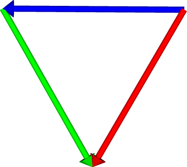
The root and minimal non-trivial weight diagrams of the algebra \(A_2 = su(3)\) are shown in Figure 2.1 The algebra has three pairs of root vectors, which are oriented east-west (colored blue), roughly northwest-southeast (colored red), and roughly northwest-southeast (colored green). The algebra's rank is the dimension of the underlying Euclidean space, which in this case is \(l=2\), and the number of non-zero root vectors is the number of raising and lowering operators. The minimal weight diagram contains six different roots, although we've only indicated one of each raising and lowering root pair. Using the root diagram, the dimension of the algebra can now be determined either from the number of non-zero roots or from the number of root vectors extending in different directions from the origin. Both diagrams indicate that the dimension of \(A_2 = su(3)\) is \(8 = 6+2\). A complex semi-simple Lie algebra can almost2 be identified by its dimension and rank. We note that the algebra's root system, and hence its root diagram or weight diagram, does determine the algebra up to isomorphism.
 |
 |
|
|
|
||
2.4 Constructing Root Diagrams from Dynkin Diagrams
In 1947, Eugene Dynkin simplified the process of classifying complex semi-simple Lie algebras by using what became known as Dynkin diagrams [9]. As pointed out above, the Killing form can be used to choose an orthonormal basis for the Cartan subalgebra. Then every root in a rank \(l\) algebra can be expressed as an integer sum or difference of \(l\) simple roots. Further, the relative lengths and interior angle between pairs of simple roots fits one of four cases. A Dynkin diagram records the configuration of an algebra's simple roots.
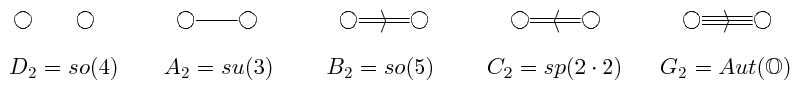
Each node in a Dynkin diagram represents one of the algebra's simple roots. Two nodes are connected by zero, one, two, or three lines when the interior angle between the roots is \(\frac{\pi}{2}\), \(\frac{2\pi}{3}\), \(\frac{3\pi}{4}\), or \(\frac{5\pi}{6}\), respectively. If two nodes are connected by \(n\) lines, then the magnitudes of the corresponding roots satisfy the ratio \(1:\sqrt{n}\). An arrow is used in the Dynkin diagram to point toward the node for the smaller root. If two roots are orthogonal, no direct information is known about their relative lengths.
We give the Dynkin diagrams for the rank 2 algebras in Figure 3 and the corresponding simple root configurations in Figure 4. For each algebra, the left node in the Dynkin diagram corresponds to the root \(r^1\) of length 1, colored red and lying along the horizontal axis, and the right node corresponds to the other root \(r^2\), colored blue.
 |
|
|
 |
||||
|
|
|
|
|
|
|
|
||||
In \(\mathbb{R}^l\), each root \(r^i\) defines an \((l-1)\)-dimensional hyperplane which contains the origin and is orthogonal to \(r^i\). A Weyl reflection for \(r^i\) reflects each of the other roots \(r^j\) across this hyperplane, producing the root \(r^k\) defined by $$r^k = r^j - 2(\frac{r^j {\tiny \bullet} r^i}{|r^i|})\frac{r^i}{|r^i|} $$ According to Jacobson [1], the full set of roots can be generated from the set of simple roots and their associated Weyl reflections.
We illustrate how the full set of roots can be obtained from the simple roots using Weyl reflections in Figure 5. We start with the two simple roots for each algebra, as given in Figure 4. For each algebra, we refer to the horizontal simple root, colored red, as \(r^1\), and the other simple root, colored blue, as \(r^2\). Step 1 shows the result of reflecting the simple roots using the Weyl reflection associated with \(r^1\). In this diagram, the black thin line represents the hyperplane orthogonal to \(r^1\), and the new resulting roots are colored green. Step 2 shows the result of reflecting this new set of roots using the Weyl reflection associated with \(r^2\). At this stage, both \(D_2 = so(4)\) and \(A_2 = su(3)\) have their full set of roots. We repeat this process again in steps 3 and 4, using the Weyl reflections associated first with \(r^1\) and then with \(r^2\). The full root systems for \(B_2 = so(5)\) and \(C_2 = sp(2\cdot 2)\) are obtained after the three Weyl reflections. Only \(G_2\) requires all four Weyl reflections.
|
|
|
|
 |
|
 |
 |
 |
||||
|
|
|
|
|
|
||||
|
|
||||||||
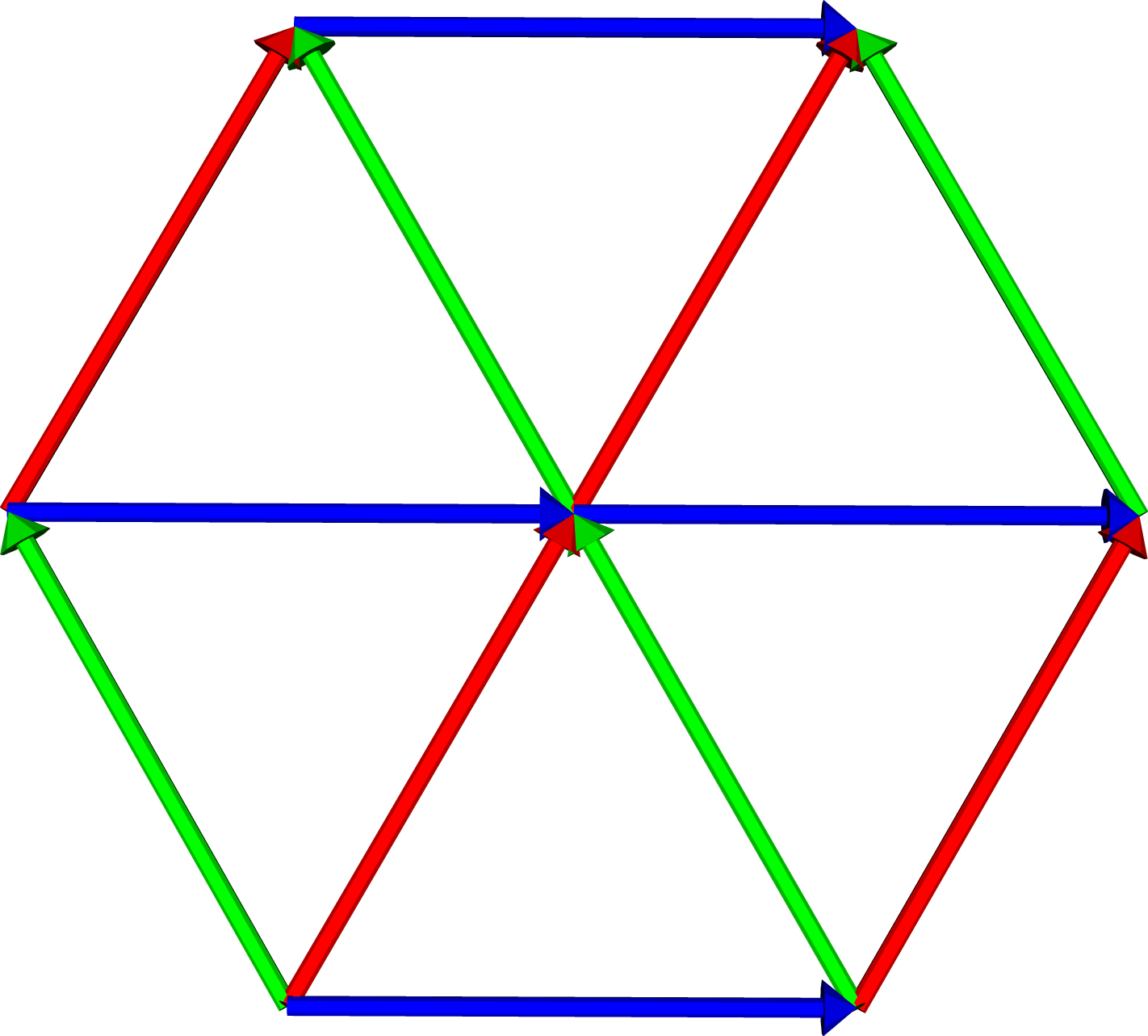
The full set of roots have been produced once the Weyl reflections fail to produce additional roots. The root diagrams are completed by connecting vertices \(r^i\) and \(r^j\) via the root \(r^k\) precisely when \(r^k + r^i = r^j\). From the root diagrams in Figure 6, it is clear that the dimension of \(A_2=su(3)\) is 8 and the dimension of \(G_2\) is 14, while both \(B_2=so(5)\) and \(C_2=sp(2\cdot 2)\) have dimension \(10\). Further, since the diagram of \(B_2\) can be obtained via a rotation and rescaling of the root diagram for \(C_2\), it is clear that \(B_2\) and \(C_2\) are isomorphic.
Tevian Dray (Oregon State Univ.) and Aaron Wangberg (Winona State Univ.), "Visualizing Lie Subalgebras using Root and Weight Diagrams," Convergence (February 2010), DOI:10.4169/loci003287


