- About MAA
- Membership
- MAA Publications
- Periodicals
- Blogs
- MAA Book Series
- MAA Press (an imprint of the AMS)
- MAA Notes
- MAA Reviews
- Mathematical Communication
- Information for Libraries
- Author Resources
- Advertise with MAA
- Meetings
- Competitions
- Programs
- Communities
- MAA Sections
- SIGMAA
- MAA Connect
- Students
- MAA Awards
- Awards Booklets
- Writing Awards
- Teaching Awards
- Service Awards
- Research Awards
- Lecture Awards
- Putnam Competition Individual and Team Winners
- D. E. Shaw Group AMC 8 Awards & Certificates
- Maryam Mirzakhani AMC 10 A Awards & Certificates
- Two Sigma AMC 10 B Awards & Certificates
- Jane Street AMC 12 A Awards & Certificates
- Akamai AMC 12 B Awards & Certificates
- High School Teachers
- News
You are here
Visualizing Lie Subalgebras using Root and Weight Diagrams
2.5 Constructing Weight Diagrams from Dynkin Diagrams
Root diagrams are a specific type of weight diagram. While the states and roots can be identified with each other in a root diagram, this does not happen for general weight diagrams. Weight diagrams are a collection of states, called weights, and the roots are used to move from one weight to another. Although it has only one root diagram, an algebra has an infinite number of weight diagrams.
Like a root diagram, any one of an algebra's weight diagrams can be constructed entirely from its Dynkin diagram. The Dynkin diagram records the relationship between the \(l\) simple roots of a rank \(l\) algebra. Each simple root \(r^1, \cdots, r^l\) is associated with a weight \(w^1, \cdots, w^l\). When all integer linear combinations of these weights are plotted in \(\mathbb{R}^l\), they form an infinite lattice of possible weights. This lattice contains every weight from every \(d \times d\) \((d \ge 0)\) representation of the algebra. These weights may be ordered. Every weight diagram then contains a highest weight \(W\) which satisfies \(W > W_i\) for every other weight \(W_i\) in the diagram. Alternatively, a diagram's highest weight \(W\) is an element of the boundary \(\overline{W}\) of the set of all weights in the diagram; \(\overline{W}\) contains all the weights in the diagram which are furthest from the origin. A particular weight diagram is chosen by selecting a weight \(W\). Weyl reflections related to the weights \(w^1, \cdots, w^l\) determine the weights in \(\overline{W}\) for the weight diagram. To determine the diagram's weights in the interior of \(\overline{W}\), we note that valid weights must be connected by the algebra's roots. Hence, all of the weights within \(\overline{W}\) which are integer linear combinations of the roots away from the weights in \(\overline{W}\) are valid and should be a part of the diagram. Having selected all of the diagram's valid weights, we complete the diagram by connecting pairs of weights with root vectors.3 Choosing a new weight \(W\) outside the original weight diagram's boundary \(\overline{W}\) selects a new, larger, weight diagram. A smaller weight diagram is created by selecting a weight contained in the interior of \(\overline{W}\).
An equivalent method [10] constructs weight diagrams while avoiding the explicit use of Weyl reflections. First, the \(l\) simple roots \(r^1, \cdots, r^l\) are used to define the Cartan matrix \(A\), whose components are \(a_{ij} = 2 \frac{r^i {\tiny \bullet} r^j}{r^i {\tiny \bullet} r^i}\). Equivalently, the components are: \[ a_{ij} =\begin{cases} 2, &\text{if $i = j$;}\\ 0, &\text{if $r^i$ and $r^j$ are orthogonal;}\\ -3, &\text{if the interior angle between $r^i$ and $r^j$ is $\frac{5\pi}{6}$, and $\sqrt{3}|r^i| = |r^j|$;}\\ -2, &\text{if the interior angle between roots $r^i$ and $r^j$ is $\frac{3\pi}{4}$, and $\sqrt{2}|r^i| = |r^j|$;}\\ -1, &\text{in all other cases;}\\ \end{cases} \]
Cartan matrices are invertible. Thus, the fundamental weights \(w^1, \cdots, w^l\) defined by \[w^i = \sum_{k=1}^{l}(A^{-1})_{ki}r^k\] are linearly independent. We create an infinite lattice \(\mathbb{W} = \{ m_i w^i | m_i \in \mathbb{Z}\}\) of possible weights in \(\mathbb{R}^l\), and then label each weight \(W^i = m^i_j w^j \in \mathbb{W}\) using the \(l\)-tuple \(M^i = \left[m^i_1, \cdots, m^i_l\right]\), called a mark. We choose one of the infinite number of weight diagrams by specifying \(l\) non-negative integers \(m^0_1, \cdots, m^0_l\) for the mark of the highest weight \(W^0\).
While the components of the Cartan matrix record the geometry of the simple roots, the components of each mark record the geometric configuration of the weights within the lattice. Each weight (W^i) is part of a shell of weights \(\overline{W}\) which are equidistant from the origin. As discussed earlier, Weyl reflections associated with the fundamental weights can be used to find the weights in \(\overline{W}\). The diagram's entire set of valid weights can also be determined using the mark \(M^i\) of each weight. The positive integers \(m^i_j \in M^i\) list the maximum number of times that the simple root \(r^j\) can be subtracted from \(W^i\) while keeping the new weights on or within the boundary \(\overline{W}\). Thus, weights \(W^i - 1 r^j, \cdots, W^i - (m^i_j) r^j \textrm{ (no sum)}\) are valid weights occurring on or inside \(\overline{W}\). These new weights have marks \(M^i - A_i^{\it{T}}, M^i - 2 A_i^{\it{T}}, \cdots, M^i - m^i_j A_i^{\it{T}}\), where \(A_i^{\it{T}}\) is the transpose of the \(i\)-th column of the Cartan matrix \(A\). Thus, given a weight diagram's highest weight \(W^0\), this procedure selects all of the diagram's weights from the infinite lattice. The diagram is completed by connecting any two weights \(W^i\) and \(W^k\) by the root \(r^j\) whenever \(W^i + r^j = W^k\).
This procedure is carried out for the the algebra \(B_3=so(7)\), whose simple roots are \[ \begin{array}{ccc} r^1 = \langle\sqrt{2},0,0\rangle, & r^2 = \langle-\sqrt{\frac{1}{2}}, -\sqrt{\frac{3}{2}}, 0\rangle, & r^3 = \langle0, \sqrt{\frac{2}{3}}, \sqrt{\frac{1}{3}}\rangle \end{array} \] We produce the Cartan matrix \(A\), find \(A^{-1}\), and list the fundamental weights.
|
|
|
|
||
| $$ A = \left( \begin{array}{ccc} 2 & -1 & 0 \\ -1 & 2 & -1 \\ 0 & -2 & 2 \end{array} \right) $$ |
|
|
Starting with the highest weight \(W^0 = w^1\), whose mark is \(\left[1,0,0\right]\), the above procedure generates the following weights:
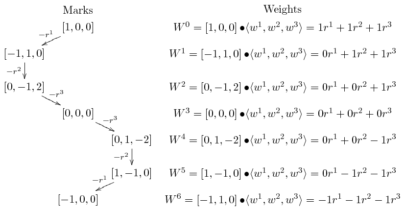
We plot the weight \(W^0, \cdots, W^6\) and the appropriate lowering roots \(-r^1, \cdots, -r^3\) at each weight for this weight diagram of \(B_3 = so(7)\) in Figure 7. The full set of roots are used to connect pairs of weights, giving the complete weight diagram of \(B_3 = so(7)\) in Figure 8.
|
|
|
|
|
|
|
2.6 Rank 3 Root and Weight Diagrams
Using the procedures outlined above, we catalog the root and minimal weight diagrams for the rank 3 algebras. We did this by writing a Perl program to generate the weight and root diagram structures and return executable Maple code. We then used Maple and Javaview to display the pictures.
The 3-dimensional root diagrams of the rank 3 algebras are given in Figure 9. The root diagrams of \(A_3=su(4)\) and \(D_3=so(6)\) are identical. Hence, \(A_3 = D_3\). These algebras have dimension 15, as their root diagram contains 12 non-zero states. The \(B_3=so(7)\) and \(C_3=sp(2\cdot 3)\) algebras both have dimension 21, and their root diagrams each contain 18 non-zero states. Each of these algebras contain the \(A_2=su(3)\) root diagram, which is a hexagon. This can be seen at the center of each rank 3 algebra by turning its root diagram in various orientations. The modeling kit ZOME [11] can be used to construct the rank 3 root diagrams. The kit contains connectors of the right length and nodes with the correct configuration of connection angles to construct all of the rank 3 root diagrams.
|
|
|
|
||
|
|
|
|
||
|
|
||||
An algebra's minimal weight diagram has the fewest number of weights while still containing all of the roots. Figure 10 shows the minimal weight diagrams for \(A_3=D_3\), \(B_3\), and \(C_3\). Each root occurs once in the diagram for \(A_3=D_3\), while in the diagram for \(B_3\) every root is used twice. The minimal weight diagram for \(C_3\) is centered about the origin, and the roots passing through the origin (colored red, blue, and brown) occur once, while the other roots occur twice.
|
|
|
|
||
|
|
|
|
||
|
|
||||
Tevian Dray (Oregon State Univ.) and Aaron Wangberg (Winona State Univ.), "Visualizing Lie Subalgebras using Root and Weight Diagrams," Convergence (February 2010), DOI:10.4169/loci003287


