- About MAA
- Membership
- MAA Publications
- Periodicals
- Blogs
- MAA Book Series
- MAA Press (an imprint of the AMS)
- MAA Notes
- MAA Reviews
- Mathematical Communication
- Information for Libraries
- Author Resources
- Advertise with MAA
- Meetings
- Competitions
- Programs
- Communities
- MAA Sections
- SIGMAA
- MAA Connect
- Students
- MAA Awards
- Awards Booklets
- Writing Awards
- Teaching Awards
- Service Awards
- Research Awards
- Lecture Awards
- Putnam Competition Individual and Team Winners
- D. E. Shaw Group AMC 8 Awards & Certificates
- Maryam Mirzakhani AMC 10 A Awards & Certificates
- Two Sigma AMC 10 B Awards & Certificates
- Jane Street AMC 12 A Awards & Certificates
- Akamai AMC 12 B Awards & Certificates
- High School Teachers
- News
You are here
Discriminants, Resultants, and Multidimensional Determinants
Publisher:
Birkhäuser
Publication Date:
2008
Number of Pages:
523
Format:
Paperback
Series:
Modern Birkhäuser Classics
Price:
39.95
ISBN:
9780817647704
Category:
Monograph
The Basic Library List Committee recommends this book for acquisition by undergraduate mathematics libraries.
[Reviewed by , on ]
David P. Roberts
10/24/2009
Israel M. Gelfand, perhaps more than any other twentieth-century mathematician, was known for the school he led. He was one of the great mathematicians who kept Soviet mathematics thriving through very difficult circumstances. MathSciNet records that Gelfand wrote more than 500 works with 150 coauthors covering 40 categories. A common theme of the Gelfand school is great depth presented in deceptively elementary language. A related theme is the use of algebraic techniques in settings such as differential equations where one might expect analytic techniques instead.
Discriminants, Resultants, and Multidimensional Determinants, joint with Mikhail M. Kapranov and Andrei V. Zelevinksy, first appeared in 1994. It is very much representative of the Gelfand school style. Discriminants and resultants of one-variable polynomials are well-known concepts, computable in a number of ways, including by ordinary determinants of square matrices. But what about the case of polynomials of more than one variable? The answer to this seemingly naive question is the elaborate and elegant theory presented in the book.
The authors are at great pains to be gentle to readers, but nonetheless I am sure that many potential readers would find the book itself intimidating. Accordingly in this review, I will highlight some important background, emphasize some of the more accessible topics, and indicate how the book fits into a larger program. I will focus on discriminants only, leaving resultants and determinants completely aside. Also the book uses "three main approaches" to its material: "a geometric approach via projective duality and associated hypersurfaces; an algebraic approach via homological algebra and determinants of complexes (Whitehead torsion); and a combinatorical approach via Newton polytopes and triangulation." The material in this review represents the third approach only.
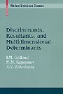
Degree. When dealing with polynomials in one variable, an important notion is degree. For example, always assuming that printed coefficients are nonzero complex numbers, the polynomial f1(x) = ax3 + bx2 + cx + d has degree three. As a warm-up to the material in the book, it is useful to reflect on how the notion of degree should be extended to polynomials in more variables. What would be the degree of say
f2(x,y) = ay2 + bx3 + cxy + d or f3(x,y) = axy2 + bx2 + cy + d?
A common response to this question would be to give the x-degree, y-degree and total degree. For f2 and f3 respectively, these numbers are (3,2,3) and (2,2,3).
This response is inadequate, as it does not fully capture the multidimensionality of the situation. To give a better response, let's first give ourselves extra flexiblity by allowing negative exponents as well. Given a Laurent polynomial f(x1,...,xm), let A ⊂ Zm be the set of exponents for which the corresponding coefficient is non-zero. A better response focuses on the Newton polytope associated to the polynomial, namely the convex hull Q of the set A of contributing exponents. Our three quadrinomial examples are illustrated by the following figure:
In this figure, the Qi are drawn in turn, with each Ai indicated by a set of four small disks. The lower left disk of each Qi is the origin of the ambient exponent space containing Qi. Each disk is drawn accompanied by its associated monomial. Thus, for example, the monomial a x y2 of f3(x,y) accompanies the top vertex of Q3 which is located at the point (1,2) of the Euclidean plane containing Q3.
In general, it is best to view the polytope Q itself as the proper higher-dimensional analog of degree. One numerical aspect of Q that is particularly important is the volume Vol(Q), with volume being normalized by Vol([0,1]m) = m! Another important numerical aspect of Q is the count #(Q), defined as the number of lattice points interior to Q. In the one-dimensional case, there is not much different between Q, Vol(Q), and #(Q): the first is an interval [u,v], the second is its length d=v–u, and the third is d–1. In higher dimensions, Q is a complicated object and Vol(Q) and #(Q) capture two of its simpler aspects. In the two-dimensional examples pictured above, one has Vol(Q2) = 6, Vol(Q3) = 5, and #(Q2) = #(Q3) = 1.
Geometry. The authors refer to the Newton polytope Q of a given Laurent polynomial f(x1,...,xm) as a "magic crystal" which sheds light on f. So before getting to the book itself, it's best to give the reader of this review some feel for this remarkable "magic."
So given f(x1,...,xm), let X be its zero-locus in the torus (C×)m. As long as the coefficients (a,b,c,...) are chosen outside of a certain discriminant locus, then X is a smooth manifold with homeomorphism type independent of the coefficients. Its real topological dimension is 2(m–1). Since it is an affine variety, its Betti numbers bi = dimQ Hi(X,Q) can be non-zero only for 0 ≤ i ≤ m–1. Its Euler characteristic χ(X) = b0 – b1 + b2 – ... + (–1)m–1bm–1 is given by the extremely simple formula
χ(X) = (–1)m–1 Vol(Q).
More subtly, but very importantly in algebraic geometry, each Betti number bi decomposes as a sum of Hodge-Deligne numbers hip,q ∈ Z≥0 satisfying the symmetry hip,q = hiq,p; here the indices p and q run over non-negative integers satisfying p+q ≤ i. The Hodge-Deligne number hm–1m–1,0 is particularly well-behaved because it doesn't change when one replaces X by any of its compactifications. This Hodge number is also known as the geometric genus g(X) of X and one has the formula
g(X) = #(Q),
valid if m > 1. Further information about Hodge-Deligne numbers can be extracted from more subtle invariants of Q.
The last paragraph can be brought thoroughly down-to-earth in the cases m = 1 and m = 2. In the case m = 1, X consists of Vol(Q) distinct points, and so χ(X) = Vol(Q) is completely evident. In the case m = 2, X is a smooth genus #(Q) curve whose canonical smooth compactification is obtained by adding one point for each segment between lattice points on the boundary of Q. Thus X2 is a genus one curve with k2 = 2 + 3 + 1 = 6 punctures while X3 is also a genus one curve, but now one with k3 = 2 + 1 + 1 + 1 = 5 punctures. In each case, the general formula relating Euler characteristic, genus, and number of punctures is satisfied: χ = 2 – 2g – k. In general for m = 2, this geometric relation holds exactly because it is the translation of Pick's theorem for convex lattice polygons. In this setting m = 2, knowledge of Hodge-Deligne numbers comes down to knowledge of (g,k). The polytope Q contains this information and very much more. So too in higher dimensions: one can expect that the combinatorial object Q goes a long way towards describing the geometric object X.
Discriminants. Finally, with some comfort with and appreciation for Q, let's move to a central focus of the book. Our starting point now is A, a finite subset of Zm. The polynomials giving rise to A as their set of contributing exponents are exactly the polynomials of the form f(x) = Σa∈A caxa for ca non-zero. Here we are using multi-index notation x=(x1,...,xm), a=(a1,...,am), and xa = x1a1... xmam. One can ask which of these give rise to a singular X. The answer is given by an explicit polynomial ΔA({ca}) ∈ Z[{ca}], well-defined up to sign. The singular X then come from exactly those polynomials f(x) = Σa∈A caxa with ΔA({ca})=0.
In the case m=1, the discriminant is computable as the resultant of f with its derivative fx. In our cubic example,
Resx(f1,f1x) = c2b2 – 4ac3 – 4b3d + 18abcd – 27a2d2 = ΔA1(a,b,c,d).
In higher-dimensional cases, a tempting approach is to iterate the one-variable process. For example, eliminating y and then x in our second example yields
Resx(Resy(f2,f2x), Resy(f2,f2y)) = –3ab2c4d(c6 – 432a3b2d) ≈ ΔA2(a,b,c,d).
Similarly, eliminating x and then y in our third example yields
Resy(Resx(f3,f3x), Resx(f3,f3y)) = 16a6b6 (27bc4 + 64a2d3) ≈ ΔA3(a,b,c,d).
As indicated by the last two displayed lines, the result of this iterative process is close to the desired discriminant. However this iteration is too naive: typically eliminating the variables in any order gets the right "main factor." However the "secondary factors" obtained from this process depend on the ordering of the variables and are often not right.
To properly define and then compute the correct ΔA, one has to be much more sophisticated in the setting m>1. Some of the ideas in the passage from A to ΔA go back to an 1848 paper of Cayley which "laid out the foundations of modern homological algebra." This "breathtaking" paper is reprinted in the back of the book and the authors say "We were happy to enter into spiritual contact with this great mathematician." Another complication, not suggested by our three examples, is that even very modest A can yield ΔA having millions of terms.
The secondary polytope. We've discussed already that the study of any given multivariate polynomial should begin with a study of its Newton polytope. Applying this principle to the polynomial ΔA, one gets its Newton polytope SA, called the secondary polytope of A. The authors write that "It was a very surprising discovery for us" when they realized that secondary polytopes "admit a very nice combinatorial description."
To describe SA, the authors describe its vertices, these being by definition in bijection with extreme monomials of ΔA. The authors find that extreme monomials are indexed by "coherent" triangulations of Q with all vertices in A. Going a step beyond SA toward ΔA itself, the authors find that the extreme monomial corresponding to a coherent triangulation T is
± ∏σ∈T Vol(σ)Vol(σ) ∏a ∈A caφT(a).
Here φT(a) is the sum of the volumes of the simplices σ incident on a.
The book presents a number of situations where the extreme monomial formula just displayed can be made much more explicit. We will present two of these situations here. The classical setting is the case when Q is one-dimensional. The setting of circuits is the case when S is one-dimensional. The one-dimensionality of one of the key polytopes, Q or S, keeps these two situations particularly simple.
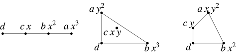
The classical case. The classical case of degree d univariate polynomials has m=1 and A = {0,1,...,d}. In the case d=3 considered above, note first that all five terms in Δ1(a,b,c,d) have total degree 4. Also if one gives a, b, c, and d weights 0, 1, 2, and 3 respectively, then all five terms have total weight 6. So the exponents i and j on the last two variables c and d determine the exponents on the first two variables a and b. We can therefore draw the secondary polytope S1 in the i–j plane as on the right below. The four A1-triangulations of the primary polytope Q1 are all coherent and drawn to the left. 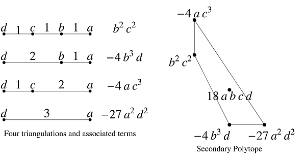
Note that the extreme-monomial formula gives four of the five terms, up to sign. Coefficients of interior terms are not covered by the theory presented in the book, and remain a mystery in general. Note also that the secondary polytope S1 is combinatorically equivalent to a square but not affinely equivalent to a square.
The case of general degree d with coefficients c0, ..., cd is similar. All terms have total degree 2d –2 . The sum of the indices on the 2d–2 factors is d(d–1). A-triangulations of Q = [0,d] are indexed by subsets of {1,...,d–1} and are all coherent. Accordingly, extreme monomials are indexed by subsets of {1,...,d–1} according to which ai appear. The monomial indexed by {1,...,d–1} itself is c12 ... cd–12 . In general, listing out the exponents which appear in increasing order, to pass from the extreme monomial indexed by a set S = {...,u,v,w,...} to the extreme monomial indexed by S – {v} = {...,u,w,...} one replaces the factor cvw–u by the factor cuw–v cwv–u. The secondary polytope is thus combinatorially an (m–1)-dimensional cube. As d = 3, 4, 5, 6, 7, ... increases, the number of terms in the discriminant increases rapidly: 5, 16, 59, 246, 1103, ...
The case of circuits. If A lies on a j-dimensional hyperplane of Zm, then one can reduce to the case of j variables. For A to not lie on a proper hyperplane one needs |A| ≥ m+1. The first case |A|=m+1 is highly non-trivial in some respects such as Hodge-Deligne numbers. However it is degenerate with respect to the discriminants and secondary polytopes, as discriminants are just 1.
The next case |A|=m+2 with A being an affine generating set for Zm is particularly interesting; in this case A is called a circuit. The vertices of the secondary polytope inside its ambient lattice can be identified with simply {0,1} inside Z. Accordingly, the discriminant ΔA then has just two terms, both given up to sign by the extreme monomial formula. The triangulations giving these terms in our second and third examples are as follows.

| ΔA2 | = | 112233a1+2b1+3c1+2+3d2+3 – 66a6b6d6 | ΔA3 | = | 1144a1+4b4c1d1+4 + 2233a3b2+3c2+3d2 |
| = | 108a3b4c6d5 – 46656 a6b6d6 | = | 256a5b4c d5 + 108a3b5c5d2 | ||
| = | 108a3b4d5 (c6 – 432a3b2d). | = | 4 a3b4c d2(27bc4 + 64a2d3). |
Thus in each case the main factor agrees with the main factor as naively calculated previously by the iterated resultant procedure.
Via simple monomial coordinates changes, the isomorphism type of the curve defined by f2(a,b,c,d;x,y)=0 depends only on t = –432a3b2c–6d. Similarly, the isomorphism type of the curve defined by f3(a,b,c,d;x,y)=0 depends only on t = –27a–1bc2d–2 The resulting one-parameter families of curves Xt are smooth for t ∈ C× except for t=1. These families are both very closely related to classical hypergeometric functions of the type 2F1(t). Similarly, a circuit in dimension m is closely related to a hypergeometric function of type mFm–1(t). The discriminant, as a function of the single variable t, is of the extremely simple form C tj(t–1).
In general, the entire theory in the book can be "quantized": to a given A, one has a system of differential equations and ΔA is only its "classical approximation." The authors are wise not to pursue this next level in the text itself, but readers should be aware that this larger theory is a primary motivation of the authors.
Conclusion. Of Gelfand's 500+ works, Discriminants, Resultants, and Multidimensional Determinants is currently the most cited on MathSciNet. A perusal of the long list of citations indicates the enormous influence of the book. Many of the citations are clearly in the framework set up by the book. Others go well beyond the book into fields as diverse as tropical geometry and mirror symmetry. Birkhäuser is not exaggerating when it calls Discriminants, Resultants, and Multidimensional Determinants a "modern classic."
David Roberts is a professor of mathematics at the University of Minnesota, Morris.
Preface.- Introduction.- General Discriminants and Resultants.- Projective Dual Varieties and General Discriminants.- The Cayley Method of Studying Discriminants.- Associated Varieties and General Resultants.- Chow Varieties.- Toric Varieties.- Newton Polytopes and Chow Polytopes.- Triangulations and Secondary Polytopes.- A-Resultants and Chow Polytopes of Toric Varieties.- A-Discriminants.- Principal A-Discriminants.- Regular A-Determinants and A-Discriminants.- Classical Discriminants and Resultants.- Discriminants and Resultants for Polynomials in One Variable.- Discriminants and Resultants for Forms in Several Variables.- Hyperdeterminants.- Appendix A. Determinants.- Appendix B. A. Cayley: On the Theory of Elimination.- Bibliography.- Notes and References.- List of Notation.- Index
- Log in to post comments


