- About MAA
- Membership
- MAA Publications
- Periodicals
- Blogs
- MAA Book Series
- MAA Press (an imprint of the AMS)
- MAA Notes
- MAA Reviews
- Mathematical Communication
- Information for Libraries
- Author Resources
- Advertise with MAA
- Meetings
- Competitions
- Programs
- Communities
- MAA Sections
- SIGMAA
- MAA Connect
- Students
- MAA Awards
- Awards Booklets
- Writing Awards
- Teaching Awards
- Service Awards
- Research Awards
- Lecture Awards
- Putnam Competition Individual and Team Winners
- D. E. Shaw Group AMC 8 Awards & Certificates
- Maryam Mirzakhani AMC 10 A Awards & Certificates
- Two Sigma AMC 10 B Awards & Certificates
- Jane Street AMC 12 A Awards & Certificates
- Akamai AMC 12 B Awards & Certificates
- High School Teachers
- News
You are here
Iterative Methods for Solving Ax = b - Convergence Analysis of Iterative Methods
On this page and the next, we attempt to answer two questions regarding the Jacobi and Gauss-Seidel Methods :


- When will each of these methods work? That is, under what conditions will they produce a sequence of approximations
x(0), x(1), x(2), … that converges to the true solution x? - When they do work, how quickly will the approximations approach the true solution? That is, what will the rate of convergence be?
so that
which we can rewrite as
where
B is often referred to as the iteration matrix.
If the current approximation x(k) is, in fact, the exact solution x, then the iterative method should certainly produce a next iteration x(k+1) that is also the exact solution. That is, it should be true that ![]() ,
,
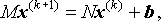
Of course, since the problem we are trying to solve is
On the other hand, choosing
To understand the convergence properties of an iterative method
we subtract it from the equation
which gives us
That is, since the current error is
![]()
To be clear, the superscript of B is the power of B, while the superscript of vector e (inside parentheses) is the iteration number to which this particular error corresponds.
Full appreciation of the significance of the relationship
Consequently, since ![]() 0
0![]() 0)
0)
We end this section by noting that one condition sometimes encountered in practice that will guarantee that
David M. Strong, "Iterative Methods for Solving [i]Ax[/i] = [i]b[/i] - Convergence Analysis of Iterative Methods," Convergence (July 2005)


