- About MAA
- Membership
- MAA Publications
- Periodicals
- Blogs
- MAA Book Series
- MAA Press (an imprint of the AMS)
- MAA Notes
- MAA Reviews
- Mathematical Communication
- Information for Libraries
- Author Resources
- Advertise with MAA
- Meetings
- Competitions
- Programs
- Communities
- MAA Sections
- SIGMAA
- MAA Connect
- Students
- MAA Awards
- Awards Booklets
- Writing Awards
- Teaching Awards
- Service Awards
- Research Awards
- Lecture Awards
- Putnam Competition Individual and Team Winners
- D. E. Shaw Group AMC 8 Awards & Certificates
- Maryam Mirzakhani AMC 10 A Awards & Certificates
- Two Sigma AMC 10 B Awards & Certificates
- Jane Street AMC 12 A Awards & Certificates
- Akamai AMC 12 B Awards & Certificates
- High School Teachers
- News
You are here
Rational Algebraic Curves: A Computer Algebra Approach

Publisher:
Springer
Publication Date:
2008
Number of Pages:
267
Format:
Hardcover
Series:
Algorithms and Computation in Mathematics 22
Price:
79.95
ISBN:
9783540737247
Category:
Monograph
[Reviewed by , on ]
David P. Roberts
05/8/2008
Algebraic geometry is a central field within mathematics which is often viewed as difficult for outsiders to enter. Recent years have seen many books which present various topics of algebraic geometry from a computational viewpoint, thereby making the subject more accessible. The book under review, RAC for short, is part of this positive trend. Its main focus is parametrizing rational plane algebraic curves. It is a graduate level text aimed at fairly wide readership, including for example readers interested primarily in computer-aided geometric design.
To give an idea of the content and level of RAC, I will slowly work out its Exercise 4.20:
Let C be the affine curve defined by
Compute a rational parametrization of C .
The problem has been posed in purely algebraic terms and, as we'll see, can be solved in purely algebraic terms. But ignoring geometry would be missing half of algebraic geometry! So we type the given polynomial into a computer algebra system to draw part of C in 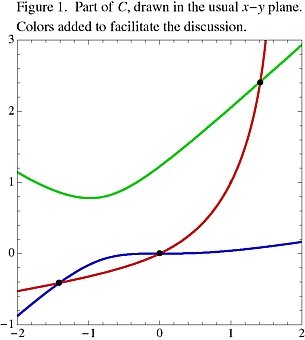 the x-y plane. We thereby obtain a monochromatic version of Figure 1. We learn immediately that at three points in this window, the curve C looks locally like the letter X. The three crossing points are called singularities, and they will play an important role in our algebraic solution. Figure 1 draws these points as small black disks.
Continuing with geometry, a problem with Figure 1 is that it shows only part of C. To remedy this problem, we can use the coordinates (u,v) = (x,y)/(r2 + x2 + y2)1/2 for any positive real r we find convenient. Via these coordinates, we can draw the entire x-y plane as the open unit disk U in the u-v plane. Exactly half the area of U comes from the disk of radius r about the origin in the x-y plane. Accordingly, one can take r small or large according to whether one wants to dedicate visual space to the part of the x-y plane near or far from the origin. In Figure 2, we view all of C in this way, taking r=3. So we learn that Figure 1 missed a whole piece of our C, the part drawn in orange at the lower right of Figure 2. In fact, Figure 1 missed this piece by a lot, since the closest the orange part of C comes to the origin is at (x,y) ≈ (20,–45).
Figure 2 has actually given us more insight than we asked of it, because the circle ∂U bounding U also plays a role. In fact, if we identify opposite points of this boundary circle then we have just abstractly sewn the closed unit diskU into the "projective plane." Our affine curve C has gained four new points to become its projective completion C.
Now let's mix algebraic and geometric thinking, as even beginning algebraic geometers should! In elementary algebraic terms, Exercise 4.20 is asking for non-constant rational functions x(t) and y(t) of minimal degree  such that f(x(t),y(t)) is identically zero. Geometrically, one can think of t as time, and then (x(t),y(t)) should be thought of as a moving point. The numbers near the curve on Figure 2 capture the solution we will be algebraically producing. At t= –∞, the point starts at the point (1,1) which is labeled ±∞ on Figure 2. Then, as t increases, the point (x(t),y(t)) moves first upwards on the red arc. It goes straight through points at infinity, and also straight through singular points, moving mostly from left to right. Finally at t=∞ the point returns to (1,1), having visited each singular point twice and all other points exactly once. Thus — despite our color scheme! — the curve C forms a single loop.
If it shocks your mathematical intuition that a plane curve C given by a random f(x,y) should be so parametrizable, then you are right! Only very special curves are parametrizable. If you are intimidated also about passing from abstract existence to actually finding (x(t),y(t)), then you are again reacting properly. In practice, it would be impossible to find (x(t),y(t)) by naive algebraic fiddling with variables. A systematic geometry-inspired approach is required, and that is the subject of RAC!
To do at least some justice to the systematic approach of RAC, let's consider a general polynomial f(x,y) with real coefficients. Let d be its degree, i.e. the largest i+j appearing among its terms axiyj. Then a sufficient condition for parametrizability is that the corresponding complete curve C consists of a single loop which crosses itself at (d–1)(d–2)/2 singular points in the x-y plane. This sufficient condition is satisfied in our case, since d=4 and (4–1)(4–2)/2=3. A weaker but similar condition, involving complex numbers among other things, is necessary and sufficient for parametrizability.
One of RAC's central algorithms is parametrization-by-adjoints in Section 4.7. Actually using this algorithm to parametrize a curve meeting our sufficient condition is a very attractive mix of algebra and geometry. The algorithm comes in several variants, as the adjoint curves involved can have degree d–2, d–1 or d. We will use the d–2 variant for our C, simultaneously indicating how it works for general d ≥ 3.
First, one locates the singularities of C by finding the common roots of f(x,y) and its partial derivatives fx(x,y) and fy(x,y). This is a standard computer algebra task. In our case, the three singularities are (0,0), (–√2,1–√2), and (√2,1+√2). Second, one chooses d–3 non-singular points of C. In our case, we need just one point and we choose (1,1). Now let V be the vector space of polynomials of degree ≤ d–2. In our case, the general element of V has the form
Let A be the subspace of V consisting of those g(x,y) which vanish on all (d–1)(d–2)/2 singular points and also on the d–3 chosen non-singular points. A key feature of this construction, expected by a naïve dimension count, is that A always has dimension two. Let g0(x,y) and g1(x,y) be a basis for A, and form the one parameter family of polynomials gt(x,y) = (1–t) g0(x,y) + t g1(x,y). In our case, suitable choices yield
Let Dt be the solution curve of gt(x,y)=0. The Dt are the adjoint curves in question. Another key feature of this construction, a consequence of Bezout's theorem this time, is that for all but finitely many t, the curves C and Dt meet at exactly one point beyond the imposed intersection points. The remaining intersection point (x(t),y(t)), unlike the imposed ones, varies with t. To find x(t), one eliminates y from the system
f(x,y) = gt(x,y)=0
and solves for x in terms of t. This is standard computer algebra, essentially a single call to a resultant command. Likewise, to find y(t) one eliminates x and solves for y. In our case, the final answer is
|
x(t) = (t–1)(t–23)(t2 + 20 t + 23)/c(t) |
|
y(t) = (t–1)3 (t–23)/c(t) |
with c(t) = t4 + 18 t 3 – 16 t 2 – 994 t – 945. We are finally done with Exercise 4.20!
As RAC rightly emphasizes, a parametrization for a curve gives one much better control over the curve than one has from a defining equation alone. For example, finding points (x,y) on our C with rational coordinates is difficult from the original description f(x,y)=0. It is trivial from the parametrization, as one can simply plug in rational t. Likewise, the colors in Figures 1 and 2 were easy to draw only after we had the parametrization. The roots of c(t) are at approximately t=–14.9, –9.2, –1.0, and 7.0; these roots serve as start and end times for our color intervals.
In some ways, RAC has a classical feel. For example, as the authors indicate, the main idea of the parametrization-by-adjoints algorithm is already present in book form in Walker's classic 1950 text. In fact, Theorem III.5.1 there gives the d–1 version. However RAC is very modern in its emphasis on computational issues. For example, the issue of solving problems like Exercise 4.20 without ever writing down computer-unfriendly irrationalities like √2 is thoroughly treated.
I am looking forward to a future when algebraic geometry has thoroughly lost its aura of inaccessibility. Books like RAC are hastening the day. If you understood this review, you are ready to read RAC. If you were annoyed at how I suppressed complex numbers, you are more than ready!
References:
Algebraic Curves , by Robert J. Walker. Dover Publications, 1950.
David Roberts is an associate professor of mathematics at the University of Minnesota, Morris.
See the table of contents in pdf format.
- Log in to post comments


