An Introduction to Population Ecology - The Logistic Growth Equation

Exponential growth can be maintained for an extended length of time only under rigid conditions (Molles, 2004). The impact of the population on the environment generally increases as a limiting resource that the population relies on decreases.

Imagine a population of deer in the forest.  They consume the various shrubbery and low leaves of trees.  At first, while the population of deer is small, there is no problem with finding enough vegetation to sustain them. However, as the population continues to increase, the vegetation becomes more difficult to find.  This creates density-dependence, which is one of the population’s intraspecific forces (Vandermeer & Goldberg, 2004).  Other intraspecific forces include competition for mates, territory, or sunlight, as well as diseases or parasites.  As a result, we have to modify the exponential growth equation to accommodate these density-dependent forces (Molles, 2004; Vandermeer & Goldberg, 2004).

Let’s suppose that the proportional rate of growth depends on the population density. Many populations in nature increase toward a stable level known as the carrying capacity, which we denote K.  The carrying capacity of a population represents the absolute maximum number of individuals in the population, based on the amount of the limiting resource available. We can incorporate the density dependence of the growth rate by using r(1 - P/K) instead of r in our differential equation:

.

 In some textbooks this same equation is written in the equivalent form

This differential equation (in either form) is called the logistic growth model. Biologists typically refer to species that follow logistic growth as K-selected species (Molles, 2004).

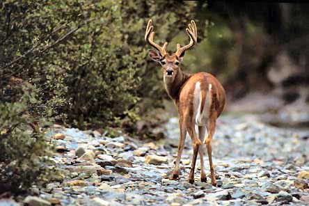
Figure 3. White-tailed deer.

Source:  Deer Stock Photography © Steven Holt/stockpix.com 
Used by permission from Stockpix.com

Example

Let’s consider the population of white-tailed deer (Odocoilus virginianus, shown in Figure 3) in the state of Kentucky. The Kentucky Department of Fish and Wildlife Resources (KDFWR) sets guidelines for hunting and fishing in the state, and it reported an estimate of 900,000 deer prior to the hunting season of 2004. Johnson (2003) notes: “A deer population that has plenty to eat and is not hunted by humans or other predators will double every three years.”  This corresponds to a rate of increase r = ln(2)/3 = 0.2311. (This assumes -- with plentiful food supply and no predation -- that the population grows exponentially, which is reasonable, at least in the short term.) The KDFWR also reports deer densities for 32 counties in Kentucky, the average of which is approximately 27 deer per square mile.  Suppose this is the deer density for the whole state (39,732 square miles). The carrying capacity K is 39,732 sq. mi. times 27 deer/sq. mi. or 1,072,764 deer.

Let’s investigate the logistic growth model by using these values in the Ecological Models Maplet -- just click on the button at the right --you need to have Maple v9.0 (or higher) installed on your machine to run this program. The maplet should open in a new window and look like Figure 4.

Figure 4. Opening Maplet Window

Choose the radio button for the Logistic Model, and click the “OK” button. A new window will appear. You can use the maplet to see the logistic model’s behavior by entering values for the initial population (P₀), carrying capacity (K), intrinsic rate of increase (r ), and a stop time.  We’ve already entered some values, so click on “Graph”, which should produce Figure 5.

We’re using mathematical units rather than biological ones. For example, 25 time units could mean 25 years or 25 minutes, depending on the biological situation. For the case of deer in Kentucky, the time units are in years, and P and K are measured in thousands.  Don’t be alarmed if you see 0.4 units for population -- in this case, that would mean 400 deer. However, you should be concerned if you see negative numbers for population!

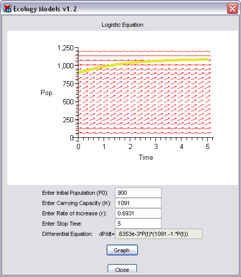
Figure 5. Maplet graph for the Logistic Model with Kentucky deer data.

Exercises

1. For the Kentucky deer population, P₀ = 900,000 deer, K = 1,072,764 deer, r = 0.2311 per year.  Describe the behavior of the population over 100 years. How does the behavior relate to the carrying capacity K?
2. Using the differential equation, find the stable equilibrium solutions. How do they relate to K?
3. Where is the graph steepest? What’s happening to the species at that time?
4. What do the red arrows represent?
5. Change the initial population P₀ to 1.2 million deer, and graph the solution again. Explain what you see.
6. Change the initial population P₀ to 500,000, and graph the solution again. Explain what you see.
7. Try using different values of K. What impact does this have on the population?
8. What if you increase the rate of increase r? What if you decrease it? Try some negative values of r. What happens to the species?
9. According to the KDFWR, Owen County, KY, had the highest population density of deer in the state in 2003 at 47 deer per square mile. Owen County is approximately 352.1 square miles. How many deer live in Owen County?
10. If 27 deer per square mile is optimal, what is the carrying capacity of Owen county? What does this tell you about the deer population?
11. Assume that the Kentucky rate of deer population increase (23.11% per year) also applies to Owen County. How many years will be required for the deer population to decrease to the Owen County carrying capacity?