- About MAA
- Membership
- MAA Publications
- Periodicals
- Blogs
- MAA Book Series
- MAA Press (an imprint of the AMS)
- MAA Notes
- MAA Reviews
- Mathematical Communication
- Information for Libraries
- Author Resources
- Advertise with MAA
- Meetings
- Competitions
- Programs
- Communities
- MAA Sections
- SIGMAA
- MAA Connect
- Students
- MAA Awards
- Awards Booklets
- Writing Awards
- Teaching Awards
- Service Awards
- Research Awards
- Lecture Awards
- Putnam Competition Individual and Team Winners
- D. E. Shaw Group AMC 8 Awards & Certificates
- Maryam Mirzakhani AMC 10 A Awards & Certificates
- Two Sigma AMC 10 B Awards & Certificates
- Jane Street AMC 12 A Awards & Certificates
- Akamai AMC 12 B Awards & Certificates
- High School Teachers
- News
You are here
The Method of Characteristics & Conservation Laws - Conservation Laws
A very important class of partial differential equations is that of conservation laws. As their name indicates, they include those equations that model the conservation laws of physics: mass, momentum, energy, etc. A scalar conservation law in one space dimension has the form
![]() , (6)
, (6)
where F(u) is a flux function. In general, conservation laws are nonlinear. For a derivation of the conservation law (6), the interested reader may consult [2, p. 31] or [3, p. 75]. We will use the method of characteristics to examine a one dimensional scalar conservation law, inviscid Burgers' equation, which takes the form of a nonlinear first order PDE. Inviscid Burgers' equation will have ![]() .
.
Inviscid Burgers' Equation
The inviscid Burgers' equation is ![]() or, equivalently,
or, equivalently, ![]() . The wave speed depends on the solution,
. The wave speed depends on the solution, ![]() . That is, the speed of a point on the solution profile will depend on the vertical coordinate u of the point. Inviscid Burgers' equation is not of the form of the linear first order PDE (1), as it is nonlinear, so our earlier analysis do not apply directly. However, from our experience with the constant coefficient (4) and variable coefficient (5) advection equations, we are led to set the characteristic equation to be
. That is, the speed of a point on the solution profile will depend on the vertical coordinate u of the point. Inviscid Burgers' equation is not of the form of the linear first order PDE (1), as it is nonlinear, so our earlier analysis do not apply directly. However, from our experience with the constant coefficient (4) and variable coefficient (5) advection equations, we are led to set the characteristic equation to be ![]() . If x(t) is a solution of this equation, then u(x(t),t) is the restriction of u to this curve. Also, along this curve,
. If x(t) is a solution of this equation, then u(x(t),t) is the restriction of u to this curve. Also, along this curve,
![]()
Thus, this solution u(x(t),t) will not change with time along the curve, so it is a characteristic curve. If we know the initial condition ![]() , we can find the characteristic curve by substituting this value into the characteristic equation
, we can find the characteristic curve by substituting this value into the characteristic equation ![]() . The right hand side of the equation is constant, indicating that the characteristic curves will be straight lines, as in the constant coefficient advection equation case. Specifically, the characteristic curve is
. The right hand side of the equation is constant, indicating that the characteristic curves will be straight lines, as in the constant coefficient advection equation case. Specifically, the characteristic curve is ![]() . The solution of the initial value problem can be written as
. The solution of the initial value problem can be written as ![]() . The solution is given implicitly and, in all but the simplest cases, it is impossible to determine the solution explicitly. The characteristics are straight lines, but the lines do not all have the same slope, so it is possible for the characteristics to intersect. If we write the characteristics as
. The solution is given implicitly and, in all but the simplest cases, it is impossible to determine the solution explicitly. The characteristics are straight lines, but the lines do not all have the same slope, so it is possible for the characteristics to intersect. If we write the characteristics as ![]() , we see that in the x-t plane they are lines with slope
, we see that in the x-t plane they are lines with slope ![]() . The slopes of the characteristics depend on the point
. The slopes of the characteristics depend on the point ![]() and on the initial data.
and on the initial data.
Unlike the first two examples, it is possible for the characteristics to intersect. If the initial data is smooth, then the method of characteristics can be used to determine the solution for small enough t such that the characteristics do not intersect. For larger t, after characteristics have intersected, the PDE will fail to have a classical solution -- that is, a single-valued solution or a function -- as the information obtained by following the characteristics will produce a multivalued solution or, possibly, no solution at all. To overcome this lack of existence of a classical solution, we must introduce a broader notion of a solution, a weak solution. Roughly speaking, a weak solution may contain discontinuities, may not be differentiable, and will require less smoothness to be considered a solution than a classical solution. Working with the weak solution of a PDE usually requires that the PDE be reformulated in an integral form. If a classical solution to the problem exists, it will also satisfy the definition of a weak solution.
If the characteristics on both sides of a discontinuity of a piecewise continuous weak solution impinge on the discontinuity curve in the direction of increasing t, the weak solution is called a shock. For inviscid Burgers' equation, the time at which the characteristics cross and a shock forms, the "breaking" time, can be determined exactly as ![]() [1, p. 25]. The formula can be used if the equation has smooth initial data (so that it is differentiable). From the formula for
[1, p. 25]. The formula can be used if the equation has smooth initial data (so that it is differentiable). From the formula for ![]() , we can see that the solution will break and a shock will form if
, we can see that the solution will break and a shock will form if ![]() is negative at some point. The discontinuous weak solution, in this case a shock wave, will travel at a speed given by the Rankine-Hugoniot condition (see [1, p. 31] and [2, p. 46]). For inviscid Burgers' equation, the shock speed s is given by
is negative at some point. The discontinuous weak solution, in this case a shock wave, will travel at a speed given by the Rankine-Hugoniot condition (see [1, p. 31] and [2, p. 46]). For inviscid Burgers' equation, the shock speed s is given by ![]() , where
, where ![]() is the value of u on the left side of a discontinuity and
is the value of u on the left side of a discontinuity and ![]() is the value of u on the right side of the discontinuity. In addition to characteristics crossing and a shock forming, there is another way the method of characteristics can break down and a discontinuity can form: The characteristics on both sides of the discontinuity can emanate from it, rather than go into it. In this case the discontinuity is called a rarefaction wave. (See the applet simulation and rarefaction example below.)
is the value of u on the right side of the discontinuity. In addition to characteristics crossing and a shock forming, there is another way the method of characteristics can break down and a discontinuity can form: The characteristics on both sides of the discontinuity can emanate from it, rather than go into it. In this case the discontinuity is called a rarefaction wave. (See the applet simulation and rarefaction example below.)
If we expand our class of solutions to include weak solutions, we no longer have uniqueness of the solution of the initial value problem, and we need an additional criterion for selecting the physically correct weak solution. This selection criterion is called an entropy condition. A different method for picking out the physically correct weak solution, but one that picks of the same weak solution as the entropy condition, is a vanishing viscosity approach.
For inviscid Burgers' equation, vanishing viscosity amounts to finding solutions to Burgers' equation, ![]() , in the limit as
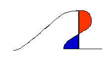
, in the limit as ![]() . A graphical technique for constructing weak solutions for problems with shocks is the equal area rule ([4, p. 42] and [1, p. 34]). Application of the equal area rule starts with the multivalued solution constructed by using the method of characteristics and then eliminates the multivalued parts by inserting shocks in a way that eliminates the multivalued solution but keeps the area under the curve the same. The equal area rule is a result of conservation. The integral of the discontinuous weak solution must be the same as the integral of the multivalued solution.
. A graphical technique for constructing weak solutions for problems with shocks is the equal area rule ([4, p. 42] and [1, p. 34]). Application of the equal area rule starts with the multivalued solution constructed by using the method of characteristics and then eliminates the multivalued parts by inserting shocks in a way that eliminates the multivalued solution but keeps the area under the curve the same. The equal area rule is a result of conservation. The integral of the discontinuous weak solution must be the same as the integral of the multivalued solution.

In the figure above, the red area is subtracted from the multivalued solution and the blue area is added. The sum of the blue and unshaded areas then makes up the weak solution. In the applet, observe in the shock problems for inviscid Burgers' equation how the plotted weak solutions appear to be applying this equal area rule to the multivalued solutions produced by the method of characteristics.
Numerical Methods for Conservation Laws
For inviscid Burgers' equation with piecewise constant initial data, we can find a formula for the weak solution. For more complicated initial data, this will most likely not be the case. Asymptotic formulas (accurate in the limit as ![]() -- see [4]) for the weak solutions to problems may exist but are of little use computationally. Thus, numerical methods that are capable of producing good approximations to the exact entropy-satisfying weak solution are important. In general, numerical methods for nonlinear hyperbolic conservation laws are more complicated and difficult to develop than numerical methods for elliptic and parabolic PDEs. For the inviscid Burgers' problem with sine wave, N-wave, and single hump initial data, the applet uses a numerical method called Roe's method to approximate the exact entropy-satisfying weak solution. This is a second order non-oscillatory finite difference method that employs the used of a flux limiter (the Superbee limiter) to suppress numerical oscillations. In the applet simulations that calculate the weak solutions by the numerical method, the ratio
-- see [4]) for the weak solutions to problems may exist but are of little use computationally. Thus, numerical methods that are capable of producing good approximations to the exact entropy-satisfying weak solution are important. In general, numerical methods for nonlinear hyperbolic conservation laws are more complicated and difficult to develop than numerical methods for elliptic and parabolic PDEs. For the inviscid Burgers' problem with sine wave, N-wave, and single hump initial data, the applet uses a numerical method called Roe's method to approximate the exact entropy-satisfying weak solution. This is a second order non-oscillatory finite difference method that employs the used of a flux limiter (the Superbee limiter) to suppress numerical oscillations. In the applet simulations that calculate the weak solutions by the numerical method, the ratio ![]() must be kept below a certain threshold, or the method will become unstable and the numerical approximations will blow up. The interested reader should consult references [1] and [3] for details.
must be kept below a certain threshold, or the method will become unstable and the numerical approximations will blow up. The interested reader should consult references [1] and [3] for details.
Inviscid Burgers' equation example problems
The following initial conditions for inviscid Burgers' equation are coded in the applet. The first two problems are Riemann problems, i.e., they have piecewise constant initial data with one discontinuity.
Riemann problem - shock
This problem has an initial condition ![]() . The characteristics intersect, and a shock forms immediately for t > 0. The exact entropy-satisfying weak solution is
. The characteristics intersect, and a shock forms immediately for t > 0. The exact entropy-satisfying weak solution is ![]() , where the shock speed is given by
, where the shock speed is given by ![]() . The exact weak solution is plotted in the applet. This problem is discussed in detail in references [1 p. 28], and [3, p. 82].
. The exact weak solution is plotted in the applet. This problem is discussed in detail in references [1 p. 28], and [3, p. 82].
Riemann problem - rarefaction
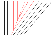
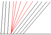
The initial condition ![]() produces characteristics (see the image below and the applet) such that there is no characteristic information available in some regions of the x-t plane.
produces characteristics (see the image below and the applet) such that there is no characteristic information available in some regions of the x-t plane.

A entropy-violating weak solution is ![]() , where s is the same as in the Riemann shock problem above. This solution corresponds to filling in the missing characteristic information as shown in red below.
, where s is the same as in the Riemann shock problem above. This solution corresponds to filling in the missing characteristic information as shown in red below.

For this problem, it can be shown that infinitely many weak solution exists [1, p. 30].
A entropy-satisfying weak solution is  . This solution corresponds to filling in the missing characteristic information as shown in red in the image below.

This problem is discussed in detail in [1 p. 28] and [3, p. 82].
Sine
The initial condition is ![]() . Notice that
. Notice that ![]() has a minimum value of
has a minimum value of ![]() . Thus, the breaking time will be
. Thus, the breaking time will be ![]() , approximately t = 0.16. This problem is discussed in detail in [3, p. 77]. The weak solution is computed by using Roe's method.
, approximately t = 0.16. This problem is discussed in detail in [3, p. 77]. The weak solution is computed by using Roe's method.
N-wave
The initial condition is ![]() . The solution consists of both a left and right moving shock. The weak solution is computed by using Roe's method. This problem is discussed in detail in [4, p. 48] and in [1, p. 32]
. The solution consists of both a left and right moving shock. The weak solution is computed by using Roe's method. This problem is discussed in detail in [4, p. 48] and in [1, p. 32]
Single hump
The initial condition is  . The solutions consist of one right-moving shock. The weak solution is computed by using Roe's method. This problem is discussed in detail in [4, p. 46].
Scott A. Sarra, "The Method of Characteristics & Conservation Laws - Conservation Laws," Convergence (September 2004)


