CalcPlot3D, an Exploration Environment for Multivariable Calculus - Lagrange Multiplier Optimization

In multivariable calculus, we teach our students the method of Lagrange multipliers to solve constrained optimization problems. As we introduce this topic, many of us use some form of visual presentation to help students understand how we develop the Lagrange multiplier equation, i.e.,

\[ \nabla f(x,y) = \lambda \nabla g(x,y)\]

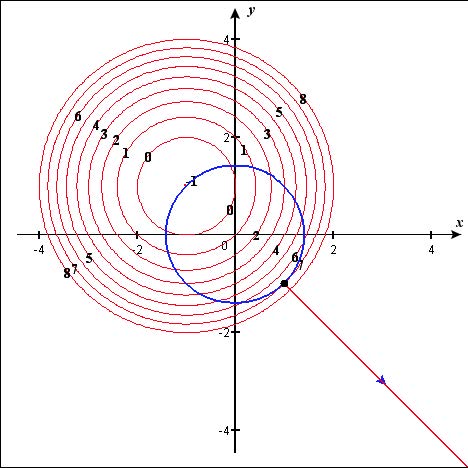
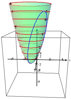
After demonstrating how this works in class with an example, I assign my students to print a visual verification of a homework problem showing both the contour plot with the constraint curve and the 3D surface plot with the constraint curve projected onto the surface showing the relative extrema visually.

Exercise: Find the relative extrema of the function f subject to the given constraint, showing all work. Then graph the function in CalcPlot3D and create its contour plot with First Level: -1, Step size: 1, and number of contours: 10. Then add the constraint curve to the plot using the Add Constraint Curve option in the Display Contour Plot dialog. Use the scrollbar at the bottom of the contour plot to move the point to one of the relative extrema. Then print the contour plot. Finally click on the contour plot and print a view of the surface (along with the contours and the constraint curve projected on the surface) that makes it possible to see both extrema clearly.

\( f(x,y)=x^2+y^2+2x-2y+1\) Constraint: \(g(x,y)=x^2+y^2=2\)

To obtain the images on the right using the applet:

1. Enter x^2 + y^2 + 2x − 2y + 1 in Function 1. Zoom out once so the x and y values range from -4 to 4.
2. To obtain the contour plot, choose the Draw Contour Plot option on the Contour Plot menu at the top of the applet.
3. On the Display Contour Plot dialog, be sure Function 1 is selected, and enter First Level: -1, Step size: 1, and number of contours: 10.
4. To display the constraint curve, select the second option on the Add Constraint Curve menu at the top of this Display Contour Plot dialog. This option is labeled, Circle centered at origin.
5. Enter 2 as \(\mathbb{R}^2\) and click on the OK button.
6. Now click on the OK button of the Display Contour Plot dialog and you should see the contour plot and the constraint curve appear.
7. By default, the gradient vectors of f and g are displayed, \(\nabla f\) is red and \(\nabla g\) is blue. To watch them vary along the constraint curve, use the scrollbar located at the bottom of the 3D plot.
8. We can visually verify that these gradient vectors are either parallel to each other or \(\nabla f=0\) when we obtain a relative extremum of f subject to the constraint, in both cases satisfying the Lagrange Multiplier equation.
9. Now click on the contour plot in the large 3D plot window. The surface above will appear. Use the right arrow key to rotate the 3D graph to the right about the z-axis until you see a clear view of the relative extrema. Then use the scrollbar again to move along the trace of the constraint curve on the surface to verify the relative extrema we found earlier.

Click here to open the CalcPlot3D applet in a new window.

Click here to open a pdf file which contains the instructions for the activity.