
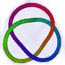
Figure 1. Trefoil Knot Diagram - Solid/Broken Lines
Knot Theory is a modern and active area of research, particularly appealing for its mathematical accessibility and visual aspect. However, knot theory also has applications of fundamental scientific significance: understanding DNA, for example. According to Sumners [18], "One of the important issues in molecular biology is the three-dimensional structure (shape) of proteins and deoxyribonucleic acid (DNA) in solution in the cell and the relationship between structure and function." The shape of DNA can be modeled by a curve. When DNA is knotted, difficulties in replication may result. Enzymes break apart and recombine DNA, affecting its structure; because the structure of DNA affects its function, understanding the types of knots formed by enzyme interactions is vital. An introduction to additional applications of knot theory can be found in [4].
Informally, we think of a knot as a curve in three-dimensional space. Formally, a knot is defined as the image of a continuous function \( f : [0, 1] \rightarrow \mathbb{R}^3 \) with the following properties:
Typically, rather than stating the function \( f \), a knot is represented by a two-dimensional image called a knot diagram. A two-dimensional projection of a knot will typically appear to have double-points -- points where the curve intersects itself. However, a knot does not intersect itself; one strand of the curve is passing over the other strand of the curve. It is particularly important to know which strand passes over the other, and knot diagrams usually convey this information in one of two ways:
These two knot diagram styles are displayed in Figure 1 and Figure 2, two knot diagrams of a trefoil knot.
Two knots are defined to be equivalent and are said to have the same knot-type if one can be continuously deformed into the other while also continuously deforming the "ambient space" -- the space surrounding the knot. (This type of transformation is known as an ambient isotopy.)
Each knot-type may be embedded in three-dimensional space in many ways, and for each embedding there are many two-dimensional projections that may be converted to a knot diagram. Thus, it is not always clear when two knots have the same knot-type. As an example, Figure 3 contains a knot diagram very different than that of Figure 1, yet these two diagrams represent equivalent knots: the trefoil knot-type.

One of the fundamental problems in knot theory is to identify the knot-type of a knot from a given image. A standard method to show that two different diagrams represent the same knot-type is by the use of the three Reidemeister moves: ways in which a knot diagram may be altered locally while preserving the knot-type of the knot [21]. If two knot diagrams represent the same knot-type, then there is a sequence of Reidemeister moves that can be used to transform one knot diagram into the other.
Finding a sequence of Reidemeister moves to show that two knots are equivalent can be complicated. Furthermore, to demonstrate that two knots represent different knot-types using this method would require a proof that no such sequence of moves exist, an even more daunting task. This difficulty motivates the idea of invariants: mathematical objects (such as numbers or polynomials) associated to a given knot-type. If one calculates a particular invariant for two knots and obtains two different answers, then the knots have different knot-types. However, the converse is false: it is possible that different knot-types may have the same value for a particular invariant.
An example of a knot invariant is the crossing number: the smallest number of crossings that appear in any diagram of the knot. For example, the crossing number of the trefoil knot is 3; any diagram of the trefoil knot has at least 3 crossings. If a knot has a diagram with fewer than three crossings, then that knot is not a trefoil. Other examples of knot invariants include: tricolorability, unknotting number, stick number, bridge number, and the Jones polynomial [1]. Some of these invariants (such as tricolorability and the Jones polynomial) can be calculated from a single knot diagram.
Topics such as knot invariants and knot equivalence can be investigated directly from knot diagrams; for many purposes, it is not necessary to know a function whose image yields the knot under investigation. However, in this article we are particularly interested in parametric functions \( f(t) = \langle \, x(t), \, y(t), \, z(t) \, \rangle \) that yield knots, specifically parameterizations whose \( x\), \(y\), and \( z \) coordinates are given by relatively simple expressions in elementary functions: polynomial or trigonometric.
Parameterizations of knots yield another source of knot invariants, arising from a "simplest" parameterization of a knot-type, just as the crossing number invariant arises from a "simplest" knot diagram of a knot-type: one with a minimal number of crossings. For example, we will consider Shastri's trefoil polynomial knot (polynomial knots wil be defined in a later section). Shastri's trefoil is the image of the function \( f(t) = \langle \, x(t), \, y(t), \, z(t) \, \rangle \) where
\[ \begin{eqnarray} x(t) &=& t^3 - 3t \\ y(t) &=& t^4 - 4t^2 \\ z(t) &=& t^5 - 10t \\ \end{eqnarray} \]The coordinate functions are polynomials of degrees 3, 4, and 5; we say that this parameterization has "degree sequence" (3, 4, 5). Although there are many other parameterizations of trefoil polynomial knots, this is the smallest degree sequence possible; any polynomial knot with a smaller degree sequence is not a trefoil.
Minimal degree sequences are invariants of polynomial knots, and furthermore, the values of this invariant are related to values of other numerical knot invariants. Therefore, it is of interest to find particularly simple parameterizations for various knot-types, and to prove that a particular parameterization is the "simplest" with which the knot-type can be attained. Results of this nature will be mentioned in the sections that follow.
Parameterizations of knots also yield another notion of equivalent knots. For a given parameterization, we replace the numerical coefficients by variables; for example, we may replace the equations of Shastri's trefoil with the equations
\[ \begin{eqnarray} x(t) &=& t^3 + at \\ y(t) &=& t^4 + bt^2 \\ z(t) &=& t^5 + ct. \\ \end{eqnarray} \]Each choice of values for the coefficients \( a\), \(b\), and \( c \) yields a curve \( f(t) = \langle \, x(t), \, y(t), \, z(t) \, \rangle \). We consider the coefficient space: the set \( S \) of values \( (a, b, c) \in \mathbb{R}^3 \) such that the curve \( f(t) \) is a polynomial knot. Following Durfee and O'Shea [6], we call two parameterized knots path-equivalent if they are in the same connected component of \( S \). In other words, two parameterized knots are path-equivalent if we can start with the parameterization of one knot, continuously vary the coefficients until we obtain the parameterization of the other knot, and all the curves corresponding to intermediate values of the coefficients are also knots (that is, we never obtain a curve that intersects itself or has a zero tangent vector at some point).
It can be shown that parameterized knots which are path-equivalent are also equivalent in the standard sense: they have the same knot-type. A question of interest is to understand the coefficient spaces for various parameterizations; for instance, determine how many connected components exist in a given coefficient space, and to what knot-types each of the components correspond.
In what follows, we introduce two families of parameterized knots (polynomial and trigonometric) and include an interactive gallery of selected knots and their equations. We survey results related to parameterizations and suggest avenues for further investigation. Finally, we include an applet that graphs three-dimensional parametric curves to aid the interested reader in exploring additional parameterizations.