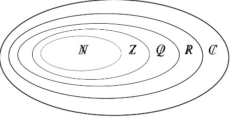
Figure 1.1: Sets of numbers
If the mathematical symbols do not show up properly within a few seconds, open the pdf-version of this chapter.
We know that some polynomial equations do not have any solutions on \(\mathbb{R}\).
Solve \(x^2 + 1 = 0\) for \(x\):
\(x^2 + 1 = 0\quad \Leftrightarrow \quad x^2 = - 1\quad \Leftrightarrow \quad x = - \sqrt { - 1} \vee x = \sqrt { - 1}\)
Problem: The equation has no solution on \(\mathbb{R}\), as \(\sqrt { - 1} \notin \mathbb{R}\).
An exit strategy is to introduce an "imaginary unit" \(i\) with \(i = \sqrt { - 1}\) or \(i^2 = - 1 \), alternatively. Then, \(x^2 + 1 = 0\) has two solutions: \(x = - i\) and \(x = i\).
Rule 1.1The imaginary unit \(i\) is defined as \(i = \sqrt { - 1}\) or \(i^2 = - 1 \). |
Solve \(x^2 - 2 \cdot x + 5 = 0\) for \(x\):
\(x^2 - 2 \cdot x + 5 = 0\quad \Leftrightarrow \quad x = - \left( {\frac{{ - 2}}{2}} \right) - \sqrt {\left( {\frac{{ - 2}}{2}} \right)^2 - 5} \vee x = - \left( {\frac{{ - 2}}{2}} \right) + \sqrt {\left( {\frac{{ - 2}}{2}} \right)^2 - 5} \quad \Leftrightarrow \quad\) \(x = 1 - \sqrt { - 4} \vee x = 1 + \sqrt { - 4} \quad \Leftrightarrow \quad\) \( x = 1 - \sqrt {4 \cdot \left( { - 1} \right)} \vee x = 1 + \sqrt {4 \cdot \left( { - 1} \right)} \quad \Leftrightarrow \quad\) \(x = 1 - 2 \cdot \sqrt { - 1} \vee x = 1 + 2 \cdot \sqrt { - 1} \quad \Leftrightarrow \quad\) \(x = 1 - 2 \cdot i \vee x = 1 + 2 \cdot i\)
The solutions \(x = 1 - 2 \cdot i\) and \(x = 1 + 2 \cdot i\) are "complex" numbers. In cartesian form they are composed from a real number and an imaginary number. Normally, complex numbers are denoted \(z\). According to the fundamental theorem of algebra, any polynomial equation of grade \(n \in \mathbb{N}\) has \(n\) complex solutions.
Rule 1.2A complex number \(z\) in cartesian form is written \(z=a+b\cdot i\) \(a, b \in \mathbb{R}\) with
|
\(z = 1 - 2 \cdot i\) and \(z = 1 + 2 \cdot i\) are the solutions of example 1.2. We have
\(a_1 = {\mathop{\rm Re}\nolimits} \left( {z_1 } \right) = 1\), \(b_1 = {\mathop{\rm Im}\nolimits} \left( {z_1 } \right) = -2\),
\(a_2 = {\mathop{\rm Re}\nolimits} \left( {z_2 } \right) = 1\), \(b_2 = {\mathop{\rm Im}\nolimits} \left( {z_2 } \right) = 2\).
Rule 1.3\(\mathbb{C}\) is the set of complex numbers \(z\). It comprises all other sets of numbers. |
Figure 1.1: Sets of numbers
Any real number \(x\) is a complex number \(z=x+0\cdot i\). Real numbers do not have imaginary units.
Rule 1.4Complex numbers are presented as points or position vectors in a cartesian diagram ("complex plane"). Any real number is located on the real axis. |
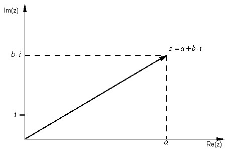
Figure 1.2: Complex plane
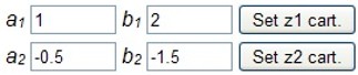
Open the Applet Basic Calculations and enter \(z_1=1+2\cdot i\) and \(z_2=-0.5-1.5\cdot i\) in cartesian form.
In studying the Applet Basic Calculations in example 1.4 you may have noticed that the complex number \(z_1=1+2\cdot i\) has also been displayed as \(z_1 = 2.2361 \cdot \exp \left( {63.4349^\circ \cdot i} \right) = 2.2361 \cdot e^{63.4349^\circ i}\). This is the so-called "exponential form" - a special case of the "polar form". Vector algebra allows us to turn any complex number \(z\) from cartesian form into polar form.
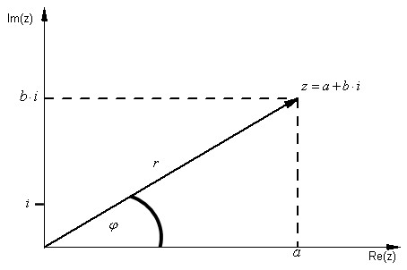
Figure 1.3: Geometric presentation of z in polar form
In order to rewrite \(z=a+b\cdot i\) in polar form we have to determine the value of \(\varphi\) and the length \(r\) of the position vector \(z=a+b\cdot i\).
Rule 1.5\(\left| z \right| \ge 0\) is the absolute value of a complex number. It corresponds the length \(r \in \mathbb{R}^{\ge 0}\) of vector \(z=a+b\cdot i\). Applying Pythagoras’ equation we get \(\left| z \right| = r = \sqrt {a^2 + b^2 }\). |
Rule 1.6\(\varphi\) is the angle between the positive real axis and the position vector \(z=a+b\cdot i\). \(\varphi\) is also called the "argument of \(z\)": \(\varphi = \arg z\). It can be given both in degree or radian. |
Due to vector algebra we have \(a = r \cdot \cos \varphi\) and \(b = r \cdot \sin \varphi\). Then, we can rewrite \(z=a+b\cdot i\) as \(z = r \cdot \cos \varphi + r \cdot i \cdot \sin \varphi = r \cdot \left( {\cos \varphi + i \cdot \sin \varphi } \right)\).
Rule 1.7\(z = r \cdot \cos \varphi + r \cdot i \cdot \sin \varphi = r \cdot \left( {\cos \varphi + i \cdot \sin \varphi } \right)\) is the "trigonometric form" of complex number \(z=a+b\cdot i\) with \(a = r \cdot \cos \varphi\) and \(b = r \cdot \sin \varphi\). |
Regarding figure 1.3 we see that \(\tan \varphi = \frac{b}{a}\) and hence
\(
\varphi = \arg z = \left\{ {\begin{array}{*{20}c}
{\arctan \frac{b}{a}\;if\;a > 0,\;b \ge 0\quad \varphi \in \left[ {0^\circ ,\;90^\circ } \right)\quad \quad \quad \;\;\;\;\;} \\
{90^\circ \;if\;a = 0,\;b > 0\quad \quad \quad \quad \quad \quad \quad \quad \quad \quad \quad \quad } \\
{180^\circ + \arctan \frac{b}{a}\;if\;a < 0\quad \varphi \in \left( {90^\circ ,\;270^\circ } \right)\quad \quad \;\;\;} \\
{270^\circ \;if\;a = 0,\;b < 0\quad \quad \quad \quad \quad \quad \quad \quad \quad \quad \quad \;\;} \\
{360^\circ + \arctan \frac{b}{a}\;if\;a > 0,\;b \le 0\quad \varphi \in \left( {270^\circ ,\;360^\circ } \right]} \\
\end{array}} \right.
\)
(degree)
or
\(
\varphi = \arg z = \left\{ {\begin{array}{*{20}c}
{\arctan \frac{b}{a}\;if\;a > 0,\;b \ge 0\quad \varphi \in \left[ {0,\;\frac{\pi }{2}} \right)\;\;\;\quad \quad \quad \;\;\;\;\;} \\
{\frac{\pi }{2}\;if\;a = 0,\;b > 0\;\;\quad \quad \quad \quad \quad \quad \quad \quad \quad \quad \quad \quad } \\
{\pi + \arctan \frac{b}{a}\;if\;a < 0\quad \varphi \in \left( {\frac{\pi }{2},\;\frac{3}{2} \cdot \pi } \right)\quad \quad \quad \quad \;\;\;} \\
{\frac{3}{2} \cdot \pi \;if\;a = 0,\;b < 0\quad \quad \quad \quad \quad \quad \quad \quad \quad \quad \quad \;\;} \\
{2 \cdot \pi + \arctan \frac{b}{a}\;if\;a > 0,\;b \le 0\quad \varphi \in \left( {\frac{3}{2} \cdot \pi ,\;2 \cdot \pi } \right]\;\;} \\
\end{array}} \right.
\)
(radian).
The trigonometric form of \(z_1=1+2\cdot i\) in example 1.4 is \(z_1 = 2.2361 \cdot \left( {\cos 63.4349^\circ + i \cdot \sin 63.4349^\circ } \right)\), as \(\varphi _1 = \arctan \frac{2}{1} = 63.4349^\circ\) and \(r_1 = \sqrt {1^2 + 2^2 } = 2.2361\).
The Euler equation enables us to convert \(z = r \cdot \left( {\cos \varphi + i \cdot \sin \varphi } \right)\) into \(z = r \cdot e^{\varphi \cdot i}\).
Rule 1.8\(z = r \cdot e^{\varphi \cdot i}\) is the exponential form of complex number \(z\). |
The polar form of \(z\) is depicted by \(r\) and \(\varphi\) . It can be displayed in either trigonometric form or exponential form. Note that it requires the trigonometric form to turn the exponential form into the cartesian form.
Throughout the following and in the applets we will prefer the exponential form to the trigonometric form, as the first one has a shorter notation and a less demanding algebra. Note that both applets display the exponential form as \(z = r \cdot \exp \left( {\varphi \cdot i} \right)\).
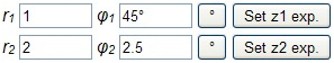
Open the Applet Basic Calculations and enter \(z_1 = 1 \cdot e^{45^\circ i} \) and \(z_2 = 2 \cdot e^{2.5 \cdot i} \) in exponential form. Note that \(\varphi _1 = \arg z_1 = 45^\circ \) is in degree, whereas \(\varphi _2 = \arg z_2 = 2.5\) is in radian. When entering \(\varphi \) in degree you have to add "°".
In order to rewrite \(z_1 = 1 \cdot e^{45^\circ i} \) and \(z_2 = 2 \cdot e^{2.5 \cdot i} \) from example 1.6 in cartesian form, one has to calculate as follows:
\(z_1 = 1 \cdot e^{45^\circ i} = 1 \cdot \left( {\cos 45^\circ + i \cdot \sin 45^\circ } \right) = 1 \cdot \left( {0.7071 + i \cdot 0.7071} \right) = 0.7071 + 0.7071 \cdot i\)Rewrite \(z = 1 + 3 \cdot i,\;z = - 1 + 3 \cdot i,\;z = - 1 - 3 \cdot i\) and \(z = 1 - 3 \cdot i\) in exponential form. Use the Applet Basic Calculations to check your answers.
Rewrite \(z = 2 \cdot e^{75^\circ i} ,\;z = e^{90^\circ i} ,\;z = 2 \cdot e^{285^\circ i}\) and \(z = \sqrt 2 \cdot e^{0.25 \cdot \pi i}\) in cartesian form. Use the Applet Basic Calculations to check your answers. You can enter \(\sqrt 2 \) as "sqrt(2)" and \(0.25 \cdot \pi\) as "0.25*pi" or "pi/4".
Dr. Jens Siebel, Last update: 08/15/2010