Leonhard Euler's totient function, \(\phi (n)\), is an important object in number theory, counting the number of positive integers less than or equal to \(n\) which are relatively prime to \(n\). It has been applied to subjects as diverse as constructible polygons and Internet cryptography. The word totient itself isn't that mysterious: it comes from the Latin word tot, meaning "so many." In a way, it is the answer to the question "Quot?" ("how many"?). In The Words of Mathematics, Steven Schwartzman [Sch] notes that question/answer pairings like Quo/To are common linguistic constructions, similar to the Wh/Th pairing in English ("Where? There. What? That. When? Then."). Beyond that, there are two key questions: (1) how did the notation emerge and develop, and (2) what questions was it originally intended to answer?

Perhaps the best way to begin this investigation is to consult some of the standard mathematical reference works. We begin with Leonard Dickson's 1919 text, History of the Theory of Numbers [Dic]. At the beginning of Chapter V, titled "Euler's Function, Generalizations; Farey Series", Dickson had two things to say about Euler:

[Euler] investigated the number \(\phi (n)\) of positive integers which are relatively prime to \(n\), without then using a functional notation for \(\phi (n)\)... Euler later used \(\pi N\) to denote \(\phi (N)\).

Each of these claims contains a footnote, the first one to Euler's paper "Demonstration of a new method in the theory of arithmetic" ([E271], written in 1758) and the second to "Speculations about certain outstanding properties of numbers" ([E564], written in 1775). So we turn to Euler.

Two Papers From Leonhard Euler

In the "Demonstration," Euler was interested in the proof of Fermat's little theorem. Interestingly, this was not the first time he had published a proof of it—his article "A proof of certain theorems regarding prime numbers" ([E54], written 1736) came first, and that proof relied on mathematical induction. Returning to the subject some 20 years later, Euler expanded on Fermat's original statement with a proof of what is today known as "Euler's theorem" or the "Euler-Fermat theorem."

Along the way, Euler effectively defined the totient function—though he did not use a mathematical notation for it. It is instead described in words, as "the multitude of numbers less than \(N\) which are prime to \(N\)." He then proved some basic facts about it, including that \(\phi(p^m) = p^{m-1}(p-1)\) for prime \(p\) [Theorem 3] and \(\phi(AB) = \phi(A)\phi(B)\) when \(A\) and \(B\) are relatively prime [Theorem 5].

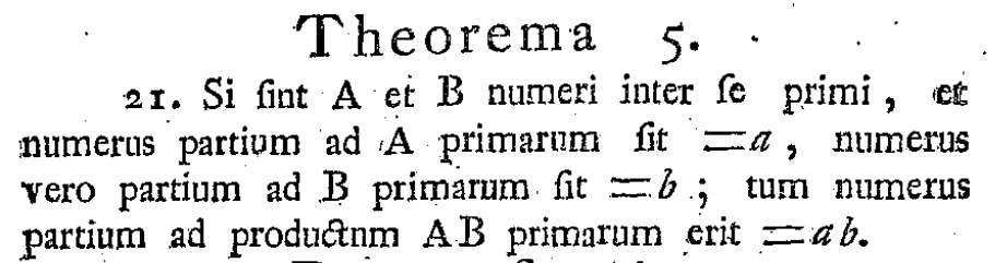
Figure 1. Theorems 3 and 5 from Leonhard Euler's paper, "Theoremata arithmetica nova methodo demonstrate" ("Demonstration of a new method in the theory of arithmetic"), published 1763. Images courtesy of the Euler Archive.

This paper is in Latin, and while Euler used the words totidem ("just as many") and tot ("so many"), they don't seem to hold any special mathematical significance. The primary result of the paper came in Theorem 11, the famed "Euler-Fermat theorem."

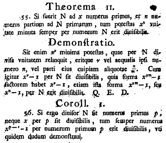
Figure 2. The Euler-Fermat theorem, appearing as Theorem 11 in Leonhard Euler's paper, "Theoremata arithmetica nova methodo demonstrate" ("Demonstration of a new method in the theory of arithmetic"), published 1763. Image courtesy of HathiTrust Digital Library.

Again, Euler only described the totient function in words, "\(n\) numerus partium ad \(N\) primarum" ("[let] \(n\) [be] the number of parts that are prime to \(N\)"). Using his terminology, \(N\) and \(x\) are relatively prime, and \(n = \phi(N)\) is the number of positive integers up to \(N\) that are relatively prime to \(N\). Theorem 11 states that \(x^n\) always has a remainder of 1 when it is divided by \(N\). Unlike Euler's earlier proof of Fermat's little theorem, the proof of this theorem relies on the factorization of polynomials.

Specifically, Euler defined \(x^\nu\) as the smallest power of \(x\) that gives remainder 1 when divided by \(N\). Relying on his previous theorem (Theorem 10), he claimed next that either \(\nu = n\) or \(\nu = \frac{n}{m}\) for some integer \(m > 1\); in other words, \(\nu\) divides \(n\). Euler then noted that, for any positive integer \(m\), \(x^\nu-1\) divides \(x^{\nu m}-1\), since 
\[
x^{\nu m}-1 = (x^\nu -1)(x^{\nu(m-1)}+x^{\nu(m-2)}+\cdots+x^\nu+1). \] Since \(n\) must be a multiple of \(\nu\) (here, \(n = \nu m\)) and \(x^\nu-1\) is divisible by \(N\), this factorization means that \(x^n - 1\) is also divisible by \(N\), which completes the proof. Immediately after this, Euler gave Fermat's original theorem as a corollary. All told, this paper lives up to its name—Euler indeed gave a demonstration of his new method for the theory of arithmetic, which produced proofs for many of the properties of the totient function.

In the "Speculations," Euler's goal was to count the number of fractions between 0 and 1 with denominators bounded above by some number \(D\). (Today this set of fractions is called a Farey sequence after the geologist John Farey, though he was almost certainly not the first to describe it.) For example, if \(D = 6\) then the list of fractions is \(\frac{1}{6},\) \(\frac{1}{5},\) \(\frac{1}{4},\) \(\frac{1}{3},\) \(\frac{2}{5},\) \(\frac{1}{2},\) \(\frac{3}{5},\) \(\frac{2}{3},\) \(\frac{3}{4},\) \(\frac{4}{5},\) \(\frac{5}{6}\), giving a total of \(11\) fractions. Since this requires one to count the number of reduced fractions for each possible denominator, the question naturally leads back to the totient function. Having decided by this time to use \(\pi\) to represent it, Euler immediately provided a table of values of \(\pi D\) for \(D\) up to 100.

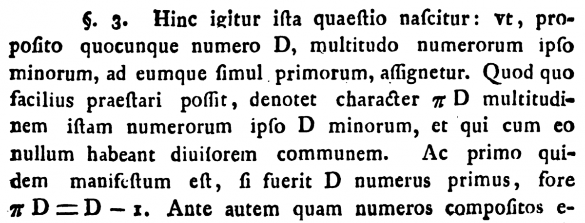
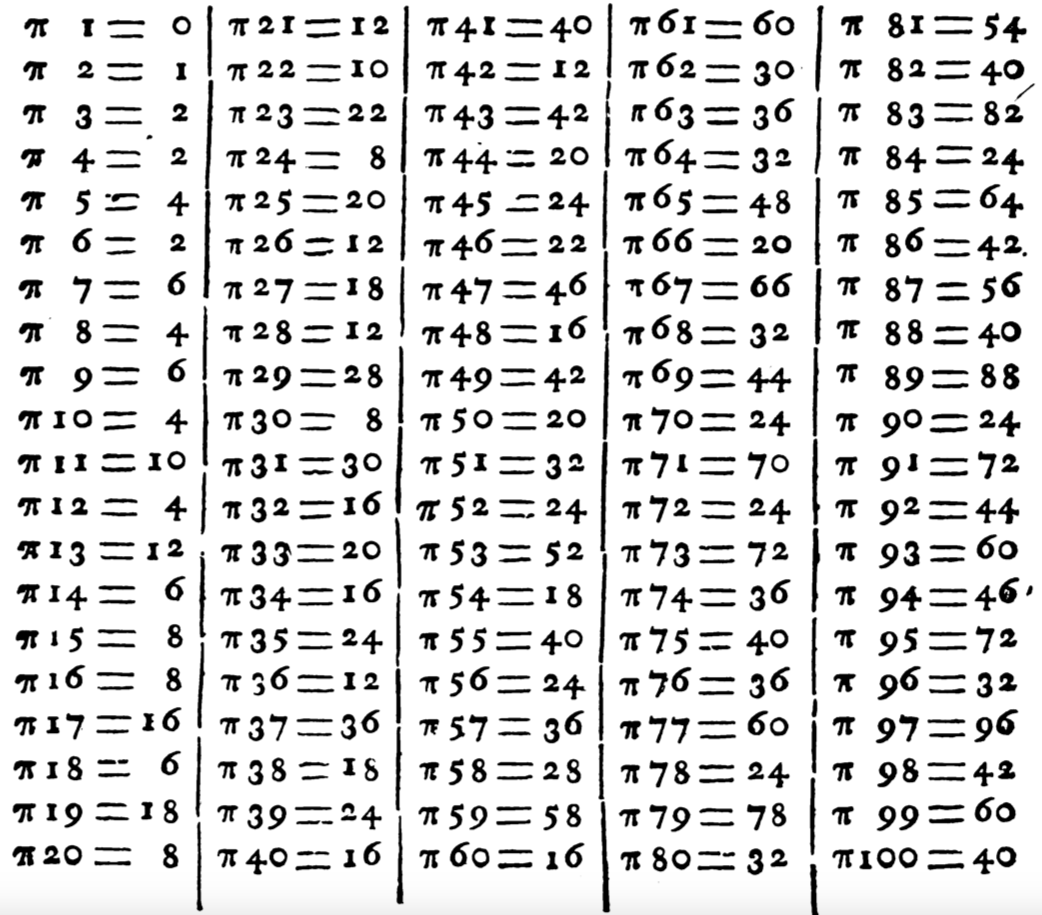
Figure 3. Euler's definition of the "character" \(\pi\), along with a table of values for \(\pi 1\) to \(\pi 100\). From "Speculationes circa quasdam insignes proprieties numerorum" ("Speculations about certain outstanding properties of numbers"), published 1784. Images courtesy of HathiTrust Digital Library.

Unlike the previous paper, here we see a clearer definition of a mathematical object. In Euler's words, "... let the character \(\pi D\) denote that multitude of numbers which are less than \(D\) and which have no common divisor with it." The reason for the extensive table is to generate a new table, this one consisting of totient sums. For example, given \(D = 6\), we find from the table that \(\pi 1 + \pi 2 + \pi 3 + \pi 4 + \pi 5 + \pi 6 = 0+1+2+2+4+2 = 11\), thus giving the number of reduced fractions between 0 and 1 which have denominator bounded above by 6. Euler compiled a table of totient sums for \(D = 10, 20, \ldots, 90, 100\).

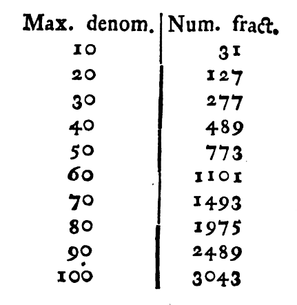
Figure 4. Euler's computation of totient sums for \(D = 10, 20, \ldots, 100\), each of which counts Farey fractions of denominator up to \(D\). From "Speculationes circa quasdam insignes proprieties numerorum" ("Speculations about certain outstanding properties of numbers"), published 1784. Images courtesy of HathiTrust Digital Library.

Euler explained the problem in general terms as follows:

... if \(D\) were the maximum denominator which we would admit, the number of all fractions will plainly be \[=1+2+3+4+\cdots+(D-1) = \frac{DD-D}{2}.\] Then all the fractions should be excluded whose value is \(\frac{1}{2}\), aside from \(\frac{1}{2}\) itself. To this end, \(D\) is divided by 2 and the quotient, either exactly or [rounded down], shall be \(=\alpha\), and it is clear that the number of fractions which are to be excluded is \(=\alpha-1\). Then for the fractions \(\frac{1}{3}\) and \(\frac{2}{3}\), let \(\frac{D}{3} = \beta\), with \(\beta\) denoting the quotient, either exactly or [rounded down], and the number of fractions to be excluded will be \(2(\beta-1) = (\beta-1)\pi 3\). In a similar way if we put \(\frac{D}{4} = \gamma\); then indeed likewise \(\frac{D}{5}=\delta\), \(\frac{D}{6} = \epsilon\), etc., as long as the quotients exceed 1, ... the multitude of fractions which are being searched for which remain will be: \[\frac{DD-D}{2} - (\alpha-1)\pi 2 - (\beta-1)\pi 3 - (\gamma-1)\pi 4 - (\delta-1)\pi 5 - etc.\]

We can see here that Euler's strategy was to begin by counting all fractions up to a given denominator, including equivalent fractions such as \(\frac{1}{2}\) and \(\frac{2}{4}\). The next step, then, would be to remove the duplicates. Euler began with those fractions equivalent to \(\frac{1}{2}\), then those equivalent to \(\frac{1}{3}\) and \(\frac{2}{3}\), and so on.

As an example, take \(D = 6\) again, so that the total number of fractions is \(1+2+3+4+5 = \frac{6^2-6}{2} = 15.\) However, the fractions \(\frac{2}{4}\), \(\frac{3}{6}\), \(\frac{2}{6}\), \(\frac{4}{6}\) all need to be removed. The first two are equal to \(\frac{1}{2}\), and can be counted using Euler's formula as \(\left(\left\lfloor\frac{D}{2}\right\rfloor - 1\right) \pi 2 = 2\cdot 1 = 2\) and \(\left(\left\lfloor\frac{D}{3}\right\rfloor - 1\right) \pi 3 = 1\cdot 2 = 2\), with \(\lfloor\cdot\rfloor\) denoting the greatest integer function. Thus, the total number of distinct fractions is \(15 - 2 - 2 = 11\), as we knew it would be. In modern terminology, we would write Euler's solution as
\[
\frac{D(D-1)}{2} - \sum_{k=2}^{\lfloor D/2\rfloor} \left(\left\lfloor\frac{D}{k}\right\rfloor - 1\right) \phi(k).
\] There is much more in this paper! Ultimately, as Euler noted, "... all of this investigation rests on this point, that, for any given number \(D\), the value of the character \(\pi D\) needs to be found." Accordingly, he repeated many of the same proofs for the totient function that he had in the "Demonstration," and improved on these results by providing a fully general formula for computing it. The interested reader can find more in Jordan Bell's English translation, which is also available via the Euler Archive.

Carl Gauss and J. J. Sylvester

Our next stop is Disquisiones Arithmeticae, Carl Gauss' 1801 number theory textbook. He conceived of this work as a thorough treatment of "higher arithmetic," accomplished by collecting together works of Euclid, Diophantus, Fermat, Euler, Lagrange, and others, and then advancing the field with new results of his own.

Gauss quickly introduced the notation \(\phi N\) to indicate the value of the totient of \(N\). On page 30, at the beginning of problem 38, he wrote:

For brevity we will designate the number of positive numbers which are relatively prime to the given number and smaller than it by the prefix \(\phi\).

This definition is immediately followed by a list of properties, including the general formula from Euler's "Speculations." 

Figure 5. Gauss' general formula in Disquisitiones Arithmeticae for computing the totient function for a given \(A\), taken from Euler's original formula in "Speculationes circa quasdam insignes proprietates numerorum" ("Speculations about certain outstanding properties of numbers"). Gauss cited Euler's work at the bottom. Image courtesy of HathiTrust Digital Library.

Gauss gave the example \(A = 60\) to illustrate the general formula. Since the factorization \(60 = 2^2\cdot 3\cdot 5\) shows that 2, 3, and 5 are the prime divisors of \(60\), the totient may be computed as 
\[
\phi\, 60 = 60 \cdot\frac{2-1}{2}\cdot\frac{3-1}{3}\cdot\frac{5-1}{5} = 60\cdot\frac{1}{2}\cdot\frac{2}{3}\cdot\frac{4}{5} = 16. \] Interestingly, this is the same example Euler gave in the "Demonstration," though to be fair, Gauss gave Euler credit for all of it.

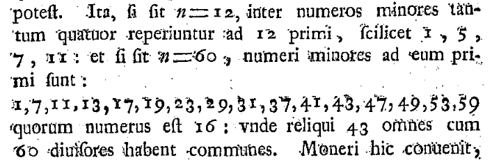
Figure 6. Euler's example from "Theoremata arithmetica nova methodo demonstrata" ("Demonstration of a new method in the theory of arithmetic"), which Gauss repeated in Disquisitiones Arithmeticae (see above). Image courtesy of the Euler Archive.

After working out the basic ideas behind his \(\phi\), Gauss' very next step was to consider a totient sum similar to Euler's. In his own words,

If \(a\), \(a'\), \(a''\) etc. are all the divisors of \(A\) (unity and \(A\) not excluded), it will be \(\phi a + \phi a' + \phi a'' + etc. = A\).

Figure 7. Gauss' totient sum from Disquisitiones Arithmeticae. Image courtesy of HathiTrust Digital Library.

Obviously, this differs from Euler's sum since Gauss only computed the sum over the divisors of \(A\). The outcome, though, is surprisingly elegant: adding the totients of a given number's divisors equals the number itself! Of course, it is Gauss' totient sum, not Euler's, that appears in most number theory textbooks today.

At this point, we should ask why Gauss used the letter \(\phi\) over Euler's \(\pi\). It's quite possible that he chose it for no particular reason. While Gauss introduced \(\phi\) for the totient early in the text, by then he had already used numerous other Greek letters. In the pages leading up to this point (at the beginning of Section II), he used \(\alpha\), \(\beta\), \(\gamma\), \(\kappa\), \(\lambda\), \(\mu\), \(\pi\), \(\delta\), \(\varepsilon\), \(\xi\), \(\nu\), \(\zeta\)—and only after these did he use \(\phi\). It is quite possible that Gauss chose the letter \(\phi\) arbitrarily, though all of the Greek letters used up to this point in the text were in service of larger ideas, and only used in the middle of a larger argument. The use \(\phi\) was new, intended to represent a general concept in number theory, so it is reasonable to wonder what Gauss' reasoning was here, especially if he had a motive for rejecting Euler's \(\pi\) notation. Unfortunately, it is impossible to determine this from the text itself.

The last major change came nearly a century later in J. J. Sylvester's article "On Certain Ternary Cubic-Form Equations," published in the American Journal of Mathematics in 1879. On page 361 Sylvester examined the specific case \(n = p^i\), where \(p\) is prime, and wrote

... \(p^{i-1}(p-1)\) is what is commonly designated as the \(\phi\) function of \(p^i\), the number of numbers less than \(p^i\) and prime to it (the so-called \(\phi\) function of any number I shall here and hereafter designate as its \(\tau\) function and call its Totient).

It is easy to miss the fact that Gauss never referred to his \(\phi\) as a function, but rather a symbol (literally, a "character"). Here we see that while Sylvester did not use today's parenthesis notation, he did refer to the totient as a function. Furthermore, while Sylvester's totient terminology has become commonplace, mathematicians continue to use \(\phi\) instead of \(\tau\). This appears to have happened in spite of Sylvester's strong preference for \(\tau\). In an 1888 paper in Nature, "Note on a Proposed Addition to the Vocabulary of Ordinary Arithmetic", Sylvester said the following about his choice of terminology for the totient function:

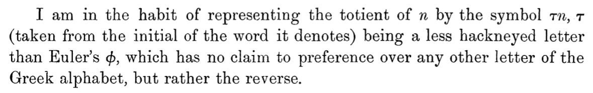
Figure 8. J. J. Sylvester's reasoning (p. 589) behind the use of \(\tau\) for the totient function. Image courtesy of the University of Michigan Historical Mathematics Collection.

Along the way, we see here that Sylvester misattributed the use of \(\phi\) to Euler, while Gauss was the true culprit. In the end, as with many things in mathematics, a well-established notation can be difficult to change even when the proposed notation is more sensible.

Conclusion

And this is where the story ends. Returning to our two original questions, we now know that the concept of a totient was due to Euler, the notation selected by Gauss, and the language for it established by Sylvester. We also know that Euler's original goals were very specific—to prove Fermat's little theorem and count fractions on the unit interval—and he proved the basic properties of the phi function as a means to these ends. More generally, we now see that the development of the totient function took quite a long time. Even though Euler's original definition appeared in 1763, it wasn't until 1801 that Gauss introduced the \(\phi\) notation and 1879 that Sylvester used the word totient to describe it—a concept 116 years in the making. Ultimately, while the original phi function was neither phi nor a function, it was undoubtedly Euler's.

References

[Dic] Dickson, Leonard. History of the Theory of Numbers, Volume I: Divisibility and Primality. Washington, DC: Carnegie Institution, 1919. (All three volumes of this text are available in paperback from Dover Publications.)

[E54] Euler, Leonhard. "Theorematum quorundam ad numeros primos spectantium demonstratio" ("A proof of certain theorems regarding prime numbers"). Commentarii academiae scientiarum Petropolitanae 8 (1741), 141–146. Numbered E54 in Eneström's index. The original text, along with an English translation by David Zhao, is available via the Euler Archive.

[E271] Euler, Leonhard. "Theoremata arithmetica nova methodo demonstrata" ("Demonstration of a new method in the theory of arithmetic"). Novi commentarii academiae scientiarum Petropolitanae 8 (1763), pp. 74–104. Numbered E271 in Eneström's index. The original text is available via the Euler Archive.

[E564] Euler, Leonhard. "Speculationes circa quasdam insignes proprietates numerorum" ("Speculations about certain outstanding properties of numbers"). Acta academiae scientarum imperialis Petropolitinae 4 (1784), pp. 18–30. Numbered E564 in Eneström's index. The original text, along with an English translation by Jordan Bell, is available via the Euler Archive.

[Gau] Gauss, Carl. Disquisitiones Arithmeticae. Leipzig: Gerhard Fleischer, 1801. An English translation by Arthur A. Clarke is available from Yale University Press, 1965.

[Sch] Schwartzman, Steven. The Words of Mathematics. Washington, DC: Mathematical Association of America, 1994.

[Syl1] Sylvester, J. J. "On Certain Ternary Cubic-Form Equations." American Journal of Mathematics 2 (1879), 357–393.

[Syl2] Sylvester, J. J. "Note on a Proposed Addition to the Vocabulary of Ordinary Arithmetic." Nature 37 (1888), 152–153.

When evaluating the speed of a computer program, it is useful to describe the long-run behavior of a function by comparing it to a simpler, elementary function. Today, we use many different notations to do this analysis, such as \(O\), \(o\), \(\Omega\), \(\ll\), and \(\sim\). Most of these notations express slightly different relationships between two functions, while some (like \(O\) and \(\ll\)) are equivalent.

More specifically, the \(f(x) \sim g(x)\) relation for two functions \(f, g : \mathbb{R} \to \mathbb{R}\) means that \(\displaystyle\lim_{x\to\infty}\) \(\frac{f(x)}{g(x)} = 1\). Under these conditions, the two functions are said to be asymptotically equivalent (or simply asymptotic). Alternatively, we say that \(f(x)\) is \(O(g(x))\) (pronounced "big-O of \(g(x)\)") if there are positive constants \(C\) and \(x_0\) such that \(|f(x)| \le C|g(x)|\) whenever \(x>x_0\). It is not too difficult to see that \(f(x) \sim g(x)\) implies that \(f(x)\) is \(O(g(x))\) and \(g(x)\) is \(O(f(x))\). The bigger question, though, is why there are so many different notations to express a relatively small number of concepts. The answer, as we will see, is that many different authors created and modified these ideas to suit their own purposes.  

German mathematician Paul Bachmann is credited with introducing the \(O\) notation to describe orders of magnitude in his 1894 book, Die Analytische Zahlentheorie (Analytic Number Theory). Before we explore Bachmann's work, though, it is worth remembering that mathematicians were certainly not the first to conceive of orders of magnitude in a quantitative sense. The English word order (and its cognates ordnung in German and ordre in French) derives from the Latin ordinem, which in medieval Europe was often used to describe a monastic society. Before that, it often referred to a series of ranked objects, such as threads in a loom or soldiers in a parade field.

By the 16th century, the word had been borrowed into the scientific vernacular, most notably by taxonomists who defined an order as a subgroup of a class. The basic idea was to rank or organize a set of diverse objects (for taxonomists, species; for mathematicians, functions) into classes of similar type. This use of the word was also picked up by astronomers, and began to appear in English in the 1850s. In one early example, Dionysius Lardner explained the vast distances encountered by an astronomer in his Hand-books of Natural Philosophy and Astronomy, published in 1859:

As spaces or times which are extremely great or extremely small are more difficult to conceive than those which are of the order of magnitude that most commonly falls under observation of the senses, we shall convey a more clear idea of velocity by selecting for our expression spaces and times of moderate rather than those of extreme length. The truth of this observation will be proved if we consider how much more clear a notion we have of the velocity of a runaway train, when we are told that it moves over fifteen yards per second... than when we are told that it moves over thirty miles an hour. We have a vivid and distinct idea of the length of fifteen yards, but a comparatively obscure [notion] of the length of thirty miles... [Lar, p. 75]

Since Lardner's goal was to provide an introduction to physics that could be "understood, without difficulty, by all persons of ordinary education" [Lar, p. 7], a discussion of this type is not surprising. In this excerpt, he asserted that velocities should be expressed with units of distance that are closer to everyday experience, owing to the difficulty in conceiving of orders of magnitude that are much larger or smaller than this. While modern readers may be skeptical that 30 miles per hour is harder to conceive of than 15 yards per second, we see here how orders of magnitude were used by astronomers as a quantitative concept before being adopted by Bachmann.

Paul Bachmann's Die Analytische Zahlentheorie

Returning to Bachmann's 1894 text, his overall goal was to present a full treatment of analytic number theory, which he conceived of as "investigations in the field of higher arithmetic which are based on analytical methods" [Bac, p. V]. In Chapter 13, Bachmann turned his attention to the analysis of number-theoretic functions, which included a basic theory for the number-of-divisors and sum-of-divisors functions. Today, these functions are often denoted by \(d(n)\) and \(\sigma(n)\). For example, the number \(n=6\) has the four divisors \(1\), \(2\), \(3\), and \(6\), so naturally \(d(6) = 4\) and \(\sigma(6) = 1+2+3+6 = 12\).

Of interest to us is the fact that Bachmann introduced the \(O\) notation at this point, in order to give a precise statement for the growth of the number-of-divisors function (which he denoted by \(T\)).

Figure 1. Bachmann's "big-O" notation, which appeared in his 1894 textbook, Die Analytische Zahlentheorie. Image courtesy of Archive.org.

Bachmann did not want to estimate the growth of \(T(n)\), but rather its summation function \(\sum_{k=1}^n T(k)\). So, if we wanted to compute \(\tau(6)\), we would need to compute all of \(T(1)\) through \(T(6)\), as shown in the table, resulting in \(\tau(6) = \sum_{k=1}^{6} T(k) = 14\).

\(n\)	1	2	3	4	5	6
\(T(n)\)	1	2	2	3	2	4

Bachmann premised his argument on the fact, proven earlier in Chapter 11, that \(\tau(n)\) can be written as \(\sum_{k=1}^n \left[\frac{n}{k}\right]\), where \(\left[x\right]\) refers to the integer part of \(x\). For \(n=6\), this would result in the sum
\[
T(6) = \left[\frac{6}{1}\right]+\left[\frac{6}{2}\right]+\left[\frac{6}{3}\right]+\left[\frac{6}{4}\right]+\left[\frac{6}{5}\right]+\left[\frac{6}{6}\right] = 6+3+2+1+1+1 = 14.
\] While this is a convenient alternative formula for \(T(n)\), Bachmann wanted an analytic estimate of its magnitude—given \(n\), roughly how large is \(T(n)\)? This formula provided the starting point for his argument, which can be seen in Figure 1. First, every rational number \(x\) can be written as \(x = [x]+\{x\}\), where \(\{x\}\) is the fractional part of \(x\). As an example, the number \(x = 1.25\) can be expressed as \(x = 1 + 0.25\), where \([x] = 1\) is the integer part and \(\{x\} = 0.25\) is the fractional part. Bachmann used \(\varrho = \{x\}\) to write \(\left[\frac{n}{k}\right] = \frac{n}{k} -\varrho\). Since each of the \(n\) terms in the sum gives rise to its own \(\varrho\) and each \(\varrho\) lies between \(0\) and \(1\), we know that \(\sum_{k=1}^n \frac{n}{k}\) differs from \(\sum_{k=1}^n \left[\frac{n}{k}\right]\) by less than \(n\). As a result,
\[
\tau(n) = \sum_{k=1}^n \left[\frac{n}{k}\right] = \sum_{k=1}^n \left(\frac{n}{k} - \varrho\right) = n\cdot \sum_{k=1}^n \frac{1}{k} - r,
\] where \(r\) is the sum of the \(\varrho\)'s and is less than \(n\). He then used a formula due to Leonhard Euler,
\[
\sum_{k=1}^n \frac{1}{k} \approx E + \log n + \frac{1}{2n},
\] where \(E \approx 0.577\) is today called the Euler-Mascheroni constant. This allowed Bachmann to reach his final conclusion of \(\tau(n) = n \log n + O(n)\). These final steps are not necessarily clear, so let's take some time to work out the details. Substituting Euler's formula into the expression for \(\tau(n)\) and rearranging the terms a bit, we find that
\[
\tau(n) = n\cdot\left(E+\log n + \frac{1}{2n}\right) - r
= n\log n + \left(E\cdot n - r + \frac{1}{2}\right).
\] Focusing on the terms in the parentheses, we can see that each of \(E\cdot n\), \(r\), and \(\frac{1}{2}\) is bounded above by a constant multiple of \(n\), so their sum must also be bounded in this way. And so we arrive at Bachmann's original conclusion, that the summation function satisfies the relation \(\tau(n) = n\log n + O(n)\). Alongside his final result, Bachmann explained that the \(O(n)\) notation referred to a quantity whose order did not exceed the order of \(n\). Unfortunately, he did not clarify this definition, even though the concept was in use throughout the remainder of the book. However, it does appear that Bachmann took the notion of "order" to be self-evident at this point in time; his imprecision is not unlike Lardner's earlier use of the word.

Edmund Landau's Handbuch

Fifteen years later, Edmund Landau published his Handbuch der Lehre von der Verteilung der Primzahlen (Handbook of the Theory of the Distribution of Prime Numbers), an attempt at a complete and systematic treatment of the main results from analytic number theory. In Section 5 of his introduction, Landau used Bachmann's \(O\) notation to express a very advanced result: estimating the number of zeroes of Riemann's zeta function with imaginary part lying in the interval \((0,T]\).

Figure 2. The first appearance of "big-O" notation in Landau's Handbuch der Lehre von der Verteilung der Primzahlen (1909). Image courtesy of the University of Michigan Digital Library.

While the precise statement goes beyond the scope of the present article, we can see that Landau's definition of the \(O\) notation differs from Bachmann's. Paraphrasing slightly, by \(O(\log T)\) Landau referred to a function of \(T\) that, when divided by \(\log T\) and taken in absolute value, will remain below a fixed upper bound for all \(T\) past a certain (possibly unknown) point. This is more precise than Bachmann's definition, and gets us very close to the definition given at the beginning of this article. The only thing missing is a formalized notation for the concepts. Not one to leave the reader wanting, Landau followed up immediately with a more formal definition.

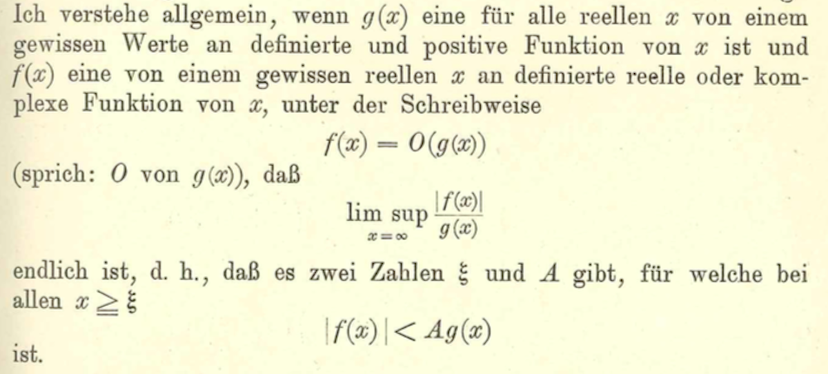
Figure 3. Landau's definition for "big-O" notation, in Handbuch der Lehre von der Verteilung der Primzahlen (1909). Image courtesy of the University of Michigan Digital Library.

Landau's final statement comes the closest to our original definition of the \(O\) notation, specifically: \(f(x)\) is \(O(g(x))\) if there exist constants \(\xi\) and \(A\) such that for all \(x\ge\xi\), \(|f(x)|<A g(x)\). In other words, \(|f(x)|\) is eventually bounded above by a constant multiple of \(g(x)\).

Landau continued more systematically in Chapter 3, at which point he developed the properties for \(O\) notation and gave definitions for both \(o\) and \(\sim\) notations.

Figure 4. Landau's definitions for "little-o" and \(\sim\) notation. Images courtesy of the University of Michigan Digital Library.

While we have not yet seen the \(o\) ("little-o") notation here, both definitions conform to what we see in contemporary mathematics. It should also be noted that Landau [Lan, p. 883] gave credit to Bachmann for the \(O\) notation:

The sign \(O(g(x))\) I found first from Mr. Bachmann (1, S. 401). The \(o(g(x))\) [notation] added here corresponds to what I used to refer to in my papers with \(\{g(x)\}\).

This concludes the development for one set of notations for orders of magnitude: \(O\), \(o\), and \(\sim\). To identify the origins for some of the other notations, we follow a different historical thread that will lead us from Germany to the United Kingdom.

G. H. Hardy and Orders of Infinity: the 'Infinitärcalcül' of Paul Du Bois-Reymond

In 1877, seventeen years before Bachmann's Die Analytische Zahlentheorie appeared in print, a paper by Paul du Bois-Reymond, "Ueber die Paradoxen des Infinitärcalcüls" ("On the paradoxical infinitary calculus"), was published in Mathematische Annalen. Du Bois-Reymond was interested in providing a rigorous foundation for Calculus, and resolving the numerous apparent paradoxes that followed from the concept of infinity (especially the infinitely small). This paper was succeeded five years later by a more ambitious work, Die allgemeine Functionentheorie (The General Theory of Functions), but we can already see some new notation appearing at this early stage.

The underlying concept of the Infinitärcalcül is that of Unendlich, literally infiniteness, but more precisely the rate of increase of a function. For example, the functions \(x^2\) and \(e^x\) have different Unendlich since the rate of increase for the second function, \(e^x\), exceeds the rate of increase of the first function \(x^2\). As an example, du Bois-Reymond sought to place a bound on the size of an infinite sequence of ever-larger functions
\[
x^{1/2}, x^{2/3}, x^{3/4}, \ldots, x^{\frac{p}{p+1}}, \ldots,
\] where \(x\) is a positive real variable and \(p\) is a positive integer. Clearly, all of these exponents are bounded above by 1, so \(x\) is an example of a function whose size exceeds all of the others (at least when \(x > 1\)). However, du Bois-Reymond wanted to be more precise than this. He gave the rather complicated function \[x^\frac{\log\log x}{\log\log x\,+\,1}\] as his example for a bounding function. This function appears to come out of nowhere, but is not without its own logic. Matching the example with the general term \(x^{\frac{p}{p+1}}\), we see that du Bois-Reymond only needed to have \(p < \log\log x\) eventually, that is for sufficiently large values of \(x\), in order to reach his desired conclusion. And since \(x\) is unbounded, it is easy to see that the inequality holds as long as \(x > e^{e^p}\). So eventually, \(x^\frac{\log\log x}{\log\log x + 1}\) will exceed any particular function in the sequence. Du Bois-Reymond represented this relationship as \[x^{\frac{p}{p+1}} \prec x^\frac{\log\log x}{\log\log x + 1} \prec x,\] with the symbol \(\prec\) indicating that each function had a larger Unendlich than the one before.

Having read du Bois-Reymond's paper, and possibly also his book Die allgemeine Functionentheorie, G. H. Hardy picked up this notation and elaborated on it in his 1910 book, Orders of Infinity: the 'Infinitärcalcül' of Paul Du Bois-Reymond. This is a short book (about 60 pages in length) whose purpose was "to bring the Infinitärcalcül up to date, stating explicitly and proving carefully a number of general theorems the truth of which Du Bois-Reymond seems to have tacitly assumed..." Hardy was also interested in how orders of growth are relevant from the student's perspective, as described in his introduction.

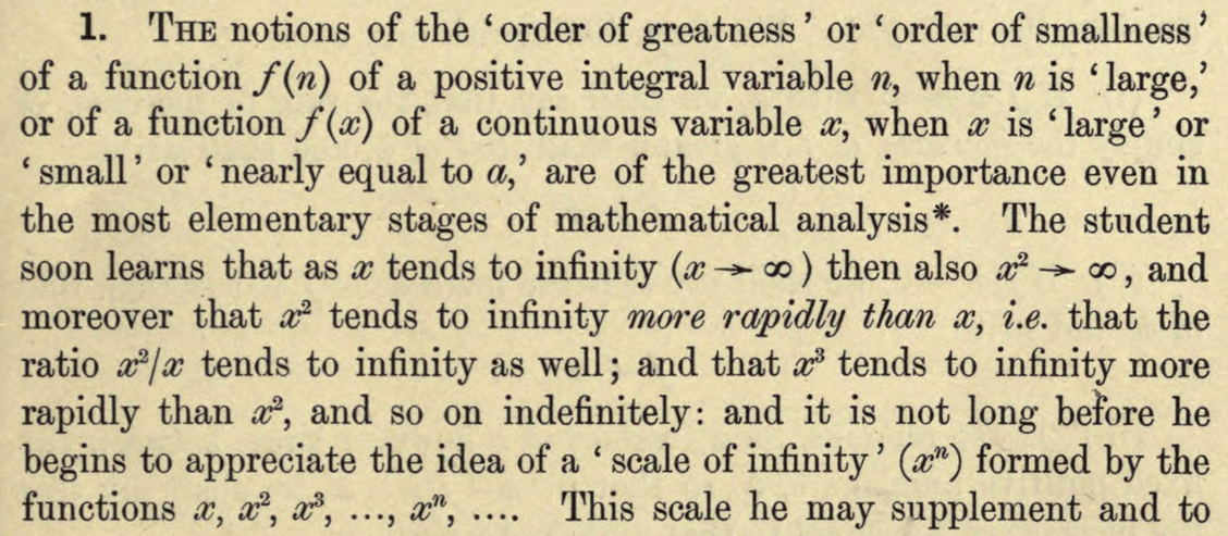
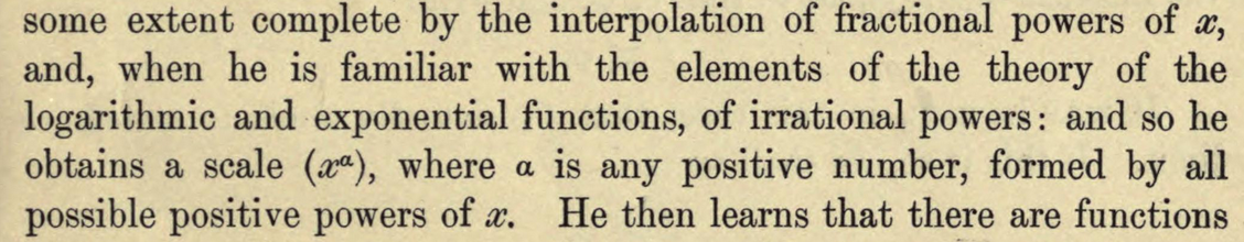
Figure 5. G. H. Hardy's motivation for studying orders of growth, from Orders of Infinity: the 'Infinitärcalcül' of Paul Du Bois-Reymond (1910). Image courtesy of Archive.org.

Hardy's goal, then, was to refine Du Bois-Reymond's notion of Unendlich to benefit students of analysis. True to his word, Hardy followed on his initial comments with a comprehensive set of definitions to clarify his notion of "order of greatness," as seen below.

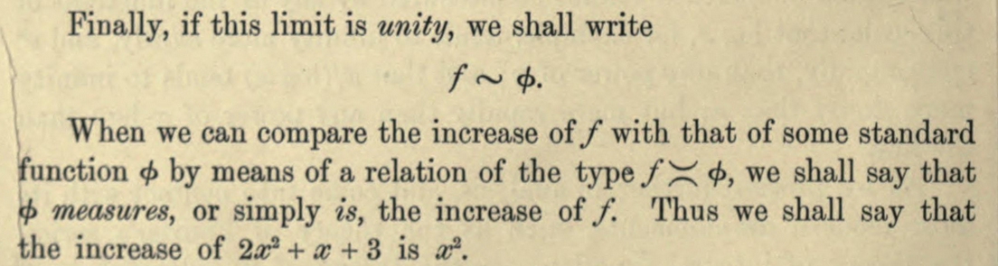
Figure 6. Hardy's use of \(\succ\), \(\prec\), and \(\asymp\) notations, from Orders of Infinity: the 'Infinitärcalcül' of Paul Du Bois-Reymond (1910). Images courtesy of Archive.org.

Clearly, the \(\prec\) notation was borrowed from Du Bois-Reymond, though today it is not typically used to compare orders of growth. Hardy also used \(\asymp\) instead of the more modern "big Theta" notation \(\Theta\), which was promoted by Donald Knuth [Knu] in the 1970s. However, we do continue to use the \(\sim\) notation (apparently borrowed from Landau) to indicate that the limit of ratios is equal to 1.

Hardy's next step was to establish a set of basic properties that would allow a student to easily assess and compare orders of growth.

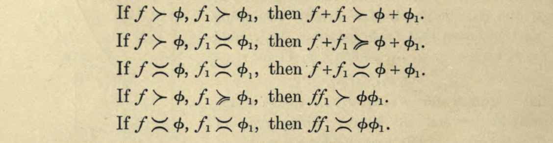
Figure 7. Elementary results about Hardy's asymptotic notations in Orders of Infinity: the 'Infinitärcalcül' of Paul Du Bois-Reymond (1910). Images courtesy of Archive.org.

Having left these proofs to the reader, Hardy then turned to Landau's \(O\) notation.

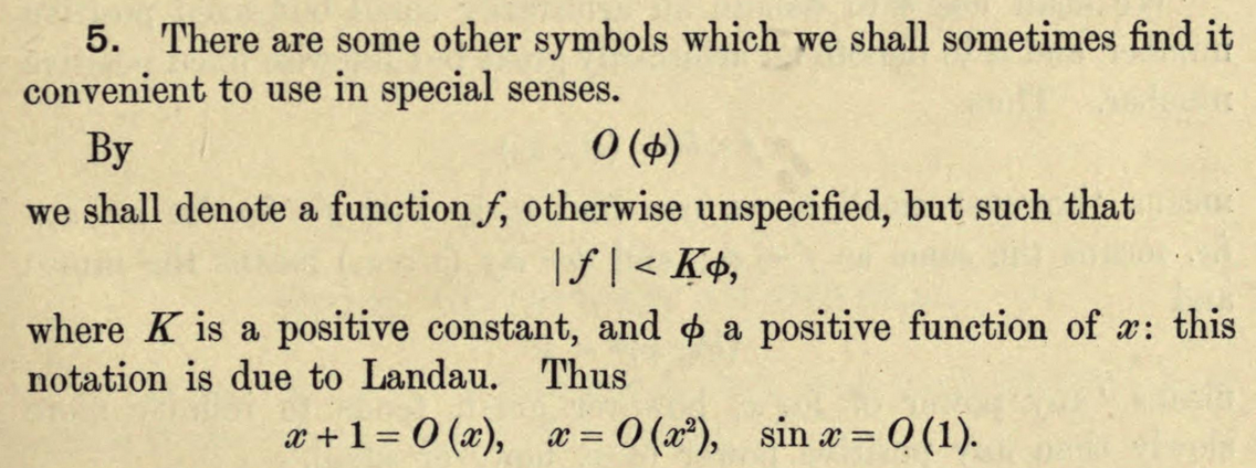
Figure 8. Hardy's definition for "big-O" notation in Orders of Infinity: the 'Infinitärcalcül' of Paul Du Bois-Reymond (1910). Interestingly, Hardy gave credit to Landau, though Bachmann had used the notation several years earlier. Image courtesy of Archive.org.

It is interesting that, in spite of his clear desire to develop a comprehensive set of notations to describe orders of growth, Hardy still introduced the big-O notation here. Looking back to his definition for \(\asymp\), we can see that using \(O\) is equivalent to using only the upper bound in \(\asymp\). Clearly, he was familiar with Landau's work and felt the notation was either useful or common enough to merit inclusion here. It also appears that he was unaware that Landau himself borrowed the big-O notation from Bachmann.

One may wonder justifiably why, given that previous notations existed, Hardy chose to attempt this revision at all. Indeed, one early review of Orders of Infinity addressed this exact issue. In his review of the book for the Bulletin of the American Mathematical Society [Hur], W. A. Hurwitz wrote:

One is impelled to wonder how much of the fairly extensive notation introduced will be found really desirable in actual use of the results. The notations of inferior and superior limit have won a permanent place; Landau's symbols \(O(f)\) and \(o(f)\) have in a short time come into such wide use as apparently to insure their retention. It is doubtful whether any further notation will be found necessary.

As is often the case, a notational choice can quickly become entrenched, and potential improvements are often cast aside in favor of a familiar—if inelegant—system. One final note here: twenty-four years later, Ivan Vinogradov [Vin] used the notation \(f(x) \ll g(x)\) as yet another alternative to writing \(f(x) = O(g(x))\). Unlike some of Hardy's symbols, this one continues to be used today.

Conclusion

So, while the notations for orders of growth were originally developed by analytic number theorists in the late 19th century, they came to be used by analysts in the early 20th century, and were adopted by computer scientists in the late 20th century. Moreover, the differing choices of these individuals led to a several different ways of expressing similar ideas. For example, we know that the expressions \(f(x) = O(g(x))\) and \(f(x) \ll g(x)\) have the same meaning, with the \(\ll\) having been introduced by Landau in 1909 and Vinogradov in 1934, respectively. Additionally, the expressions \(f(x) = \Theta(g(x))\) and \(f(x) \asymp g(x)\) have the same meaning, though the former was due to Hardy in 1910, while the latter came into use due to Knuth in the 1970s. While Landau's "big-O" notation was adopted early, the varied interests of scholars gave space for redundant or nuanced terms to be defined as circumstances dictated. Undoubtedly, not all mathematics is developed in a clean and concise way, and here we see that the path to new mathematical truths can be a meandering one.

References

[Bac] Bachmann, Paul. Die analytische Zahlentheorie. Leipzig: Teubner, 1894.

[duB] du Bois-Reymond, Paul. "Ueber die Paradoxen des Infinitärcalcüls." Math. Ann. (June 1877) 11, Issue 2, 149-167.

[Har] Hardy, G. H. Orders of Infinity: the "Infinitärcalcül" of Paul Du Bois-Reymond. Cambridge University Press, 1910.

[Hur] Hurwitz, Wallie A. Review: G. H. Hardy, Orders of Infinity. The "Infinitärcalcül" of Paul Du Bois-Reymond. Bull. Amer. Math. Soc. 21, No. 4 (1915), 201-202.

[Knu] Knuth, Donald. "Big Omicron and Big Theta and Big Omega." SIGACT News (April-June 1976) 8, Issue 2, 18-24.

[Lan] Landau, Edmund. Handbuch der Lehre von der Verteilung der Primzahlen. Leipzig: Teubner, 1909.

[Lar] Larder, Dionysius. Hand-books of Natural Philosophy and Astronomy. Philadelphia: Blanchard and Lea, 1859.

[Vin] I. M. Vinogradov. "A new estimate for \(G(n)\) in Waring's problem" Dokl. Akad. Nauk SSSR 5 (1934), 249–253.

In most undergraduate linear algebra courses, eigenvalues (and their cousins, the eigenvectors) play a prominent role. Their most immediate application is in transformational geometry, but they also appear in quantum mechanics, geology, and acoustics. Those familiar with the subject will know that a linear transformation \(T\) of an \(n\)-dimensional vector space can be represented by an \(n\times n\) matrix, say \(M,\) and that a nonzero vector \(\vec{v}\) is an eigenvector of \(M\) if there is a scalar \(\lambda\) for which \[M\vec{v} = \lambda\vec{v}.\] Narrowing our focus to \(n\)-dimensional real space, we may take \(I\) to be the \(n\times n\) identity matrix, in which case the equation becomes \[(\lambda I - M)\vec{v} = \vec{0}.\] This equation can hold for a nonzero vector \(\vec{v}\) (our eigenvector) only when the determinant of \(\lambda I - M\) is zero. This leads us to a characteristic polynomial, defined by \[\det(\lambda I - M).\] Roots of this polynomial are the eigenvalues \(\lambda\) of the matrix \(M\).

As an example, consider the transformation of \(\mathbb{R}^3\) represented by the matrix \[M = \begin{bmatrix} 2 & 1 & 0 \\ 1 & 0 & 0 \\ 0 & 0 & -1 \end{bmatrix}.\] The characteristic polynomial is given by \[\det \begin{bmatrix} \lambda-2 & -1 & 0 \\ -1 & \lambda & 0 \\ 0 & 0 & \lambda+1 \end{bmatrix} = \lambda^3-\lambda^2-3\lambda-1,\] and so the eigenvalues of \(M\) are the roots \(-1\), \(1-\sqrt{2}\), \(1+\sqrt{2}\) of this polynomial. (Linear algebra students may recall that since this matrix is symmetric, we know before computing them that the eigenvalues must be real.) The respective eigenvectors are \(\langle 0,0,1\rangle\), \(\langle 1,-1-\sqrt{2},0\rangle\), \(\langle 1,-1+\sqrt{2},0\rangle\).

Now consider the words I have used here, and in particular note the presence of the German prefix eigen-. This may be perplexing to most readers, and indeed, its use in North America has not always been so common. In fact, over the past two centuries the words proper, latent, characteristic, secular, and singular have all been used as alternatives to our perplexing prefix. And while these variations have disappeared from common use in the United States, we'll see that even today the argument is not quite over.

Before going further, though, note that the prefix eigen- predates its mathematical use. Old English used the word agen to mean "owned or possessed (by)," and while this usage no longer exists in modern English, eigen is used to mean "self" in modern German. For example, the word eigenkapital is usually translated into English as equity, though a more literal translation would be "self capital." In other words, this word refers to the principal that is the borrower's own—the money that has already been payed to the lender. Interestingly, this meaning also carries over to acoustics, where an eigentöne (literally, "self-tone") is a frequency that produces resonance in a room or other performance space. So we can see that the prefix eigen- had a well-established usage in German (and once upon a time, in English). How, then, did it get attached to mathematics?

Cauchy and Celestial Mechanics

The proper mathematical history of the eigenvalue begins with celestial mechanics, in particular with Augustin-Louis Cauchy's 1829 paper "Sur l'équation à l'aide de laquelle on détermine les inégalités séculaires des mouvements des planétes" ("On the equation which helps one determine the secular inequalities in the movements of the planets"). This paper, which later appeared in his Exercises de mathématiques [Cau1], concerned the observed motion of the planets. At this time, astronomers and mathematicians were making detailed observations of the planets in order to validate the mathematical models inherited from Kepler and Newton's laws of motion. One famous outcome of this program was Urbain Le Verrier's prediction of the existence of Neptune based on observed perturbations in the orbit of Uranus.

In celestial mechanics, most perturbations are periodic; for example, Neptune's influence on Uranus's orbit waxes and wanes as the planets revolve around the sun. However, one perplexing issue in the 18th and 19th centuries was that of secular perturbations—those non-periodic perturbations that increase gradually over time. Today, the word secular usually refers to those aspects of society and culture that are not religious or spiritual in nature. However, it also carries the meaning of something whose existence persists over long stretches of time (coming from the Latin saecularis, "occurring once in an age"), which is the more accurate usage in this case. As it happens, Cauchy's original interest in this subject was not secular perturbation, but rather the axes of motion for certain surfaces in three dimensional space. In an 1826 note to the Paris Academy of Sciences, Cauchy wrote:

It is known that the determination of the axes of a surface of the second degree or of the principal axes and moments of inertia of a solid body depend on an equation of the third degree, the three roots of which are necessarily real. However, geometers have succeeded in demonstrating the reality of the three roots by indirect means only... The question that I proposed to myself consists in establishing the reality of the roots directly... [Haw1, p. 20]

In today's language, we would say that Cauchy's research program was to show that a symmetric matrix has real eigenvalues. When "Sur l'équation" appeared in print three years later, Cauchy had succeeded in a direct proof of this fact. His argument began by establishing some basic properties for a real, homogeneous function of degree two in \(\mathbb{R}^n\). (For simplicity, we will only consider the three-dimensional version of the problem.)

Figure 1. In "Sur l'équation à l'aide de laquelle on détermine les inégalités séculaires des mouvements des planétes" (1829), Cauchy used the Lagrange multiplier method to begin his eigenvalue problem. Image courtesy of the Bibliothèque Nationale de France's Gallica collection.

Cauchy restricted his function to the unit sphere, in which case its maxima and minima on the unit sphere may be found via the equation \[\frac{\varphi(x,y,z)}{x} = \frac{\chi(x,y,z)}{y} = \frac{\psi(x,y,z)}{z},\] where \(\varphi = \frac{\partial f}{\partial x}\), \(\chi = \frac{\partial f}{\partial y}\), and \(\psi = \frac{\partial f}{\partial z}\). (Readers might recognize this as the Lagrange multiplier method found in most multivariable calculus courses.) Next, he defined the quantities \(A_{xx}\), \(A_{xy}\), \(A_{yx}\), etc., according to the coefficients on the terms \(x^2\), \(xy\), \(yx\), etc. (Note that the pure second-order partial derivatives are equal to their corresponding \(A\) value, but in Cauchy's notation mixed partials are twice the corresponding \(A\) value.) Using the fact that \(A_{xy} = A_{yx}\), Cauchy obtained a system of equations that gave a solution to the eigenvalue problem.

Figure 2. Cauchy's method for determining extrema for a real, homogeneous function of degree two restricted to the unit sphere in \(\mathbb{R}^n\), from "Sur l'équation à l'aide de laquelle on détermine les inégalités séculaires des mouvements des planétes" (1829). Image courtesy of the Bibliothèque Nationale de France's Gallica collection.

To better illuminate the connection between Cauchy's problem and a modern eigenvalue problem, let's consider the function \(f(x,y,z) = x^2 + xy - \frac{1}{2}z^2\) on the unit sphere. The nonzero second-order partial derivatives are \(\frac{\partial^2 f}{\partial x^2} = 2\), \(\frac{\partial^2 f}{\partial z^2} = -1\), and \(\frac{\partial^2 f}{\partial x \partial y} = 1\). In matrix form, we have \[\begin{bmatrix} A_{xx} & A_{xy} & A_{xz} \\ A_{yx} & A_{yy} & A_{yz} \\ A_{zx} & A_{zy} & A_{zz} \end{bmatrix} \;=\; \begin{bmatrix} 2 & 1 & 0 \\ 1 & 0 & 0 \\ 0 & 0 & -1 \end{bmatrix},\] which is the same matrix from our earlier example.

Next, he used the determinant of the matrix (while notably using neither the word "determinant" or "matrix") to show that \(s\) must always be real. Cauchy reasoned that, if the characteristic polynomial had complex roots, they must come in conjugate pairs. Thus, there would be two \((n-1) \times (n-1)\) minors within the eigenvalue matrix whose determinants would be complex conjugates of each other. From here, Cauchy showed that the product of these determinants must be zero, i.e., the rank of the matrix is at most \(n-1\). Ultimately, his argument was a reductio ad absurdum, in which a symmetric matrix with non-real eigenvalues can be shown to have rank at most \(n-1\), then at most \(n-2\), etc., until the matrix itself vanishes. (The interested reader should take a look at the original paper, available from Gallica.)

Cauchy returned to the subject of linear equations in his 1840 paper "Mémoire sur l'integration des équations linéaires" [Cau2]. While this paper was focused on pure mathematics, his ultimate goal was to solve physics problems: "It is the integration of linear equations, and above all linear equations with constant coefficients, that is required for the solution of a large number of problems in mathematical physics." Later in the introduction, he described how to solve a system of linear differential equations using his newly-named équation caractéristique as the principal tool.

... after having used elimination to reduce the principal variables to a single one, we may, with the help of these methods, express the principal variable as a function of the independent variable and arbitrary constants, then... determine the values of the arbitrary constants, using simultaneous equations of the first degree... we obtain for the general value of the principal variable a function in which there enter along with the principal variable the roots of a certain equation that I will call the characteristic equation, the degree of this equation being precisely the order of the differential equation which is to be integrated. [Cau2, p. 53]

In the section "Intégration d'un système d'équations différentielles du premier ordre, linéaires et à coefficients constants" ("Integration of a system of linear, first-order differential equations with constant coefficients"), Cauchy described this process with a bit more detail.

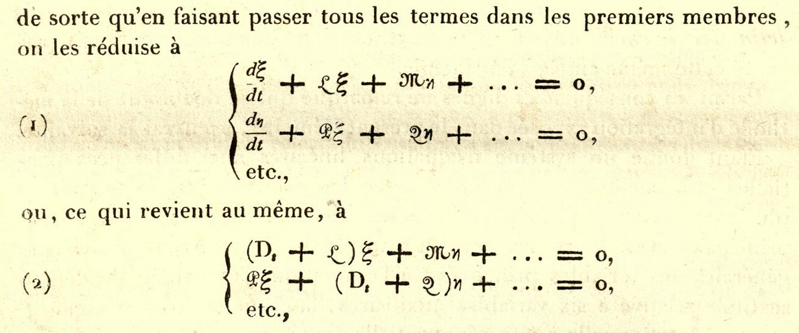
Figure 3. Cauchy's method for solving a system of linear, first-order differential equations with constant coefficients, equivalent to a modern-day eigenvalue problem. From "Mémoire sur l'integration des équations linéaires" (1840); image courtesy of Archive.org.

For the sake of clarity, let us take \(n = 3\) and apply Cauchy's reasoning to our earlier example. In this case, the differential equations are \[\begin{cases} \frac{d\xi}{dt} + 2\xi + \eta & = 0 \\ \frac{d\eta}{dt} + \xi & = 0 \\ \frac{d\zeta}{dt} - \zeta & = 0 \end{cases}.\] In our example, it is easy to see that the equation for \(\zeta\) has solution \(\zeta = Ce^t\). Untangling the first two equations takes a bit more work. Cauchy's method would set \(\xi = Ae^{st}\) and \(\eta = Be^{st}\) and substitute into the system.

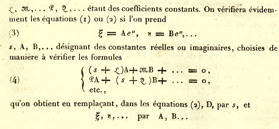
Figure 4. More of Cauchy's method for solving a system of linear, first-order differential equations with constant coefficients, equivalent to a modern-day eigenvalue problem. From "Mémoire sur l'integration des équations linéaires" (1840); image courtesy of Archive.org.

In our example, making the substitution and canceling the common term \(e^{st}\) will produce the system \[\begin{cases} (s + 2)A + B & = \; 0 \\ sB + A & = \; 0 \end{cases}\] which has nontrivial solutions when \(s = -1\pm\sqrt{2}\). Of course, we could write the whole system of differential equations in matrix form and divide by \(e^{st}\) to get \[\begin{bmatrix} s+2 & 1 & 0 \\ 1 & s & 0 \\ 0 & 0 & s-1 \end{bmatrix} \begin{bmatrix} A \\ B \\ C \end{bmatrix} = \begin{bmatrix} 0 \\ 0 \\ 0 \end{bmatrix},\] which is the same eigenvalue problem we saw at the beginning, except with \(-s\) substituted for \(\lambda\). In the general, \(n\)-dimensional case, one must reduce the system of equations via elimination to produce a degree \(n\) polynomial in \(s\). Cauchy named the equation, in which this general polynomial is set equal to \(0\), the "characteristic equation."

Figure 5. The conclusion of Cauchy's method for solving a system of linear, first-order differential equations with constant coefficients, including his naming of the équation caractéristique. From "Mémoire sur l'integration des équations linéaires" (1840); image courtesy of Archive.org.

We can easily see how Cauchy's method of solution is equivalent to a modern eigenvalue problem from a typical linear algebra course. As an aside, note that Cauchy referred to the eigenvalues as valeurs propres (proper values) near the end of this passage.

Latent and Singular Values

In 1846, only six years after Cauchy's "Mémoire sur l'integration des équations linéaires" appeared in print, Johann Gottfried Galle observed an object in the night sky from the Berlin observatory, roughly in the place that Le Verrier had predicted it would be found. Six years later, J. J. Sylvester published a seemingly-unrelated note in Philosophical Magazine on the use of matrices in solving homogeneous quadratic polynomials. In this paper, Sylvester used no terminology for the eigenvalues of a matrix, merely calling them "roots" of a determinant equation.

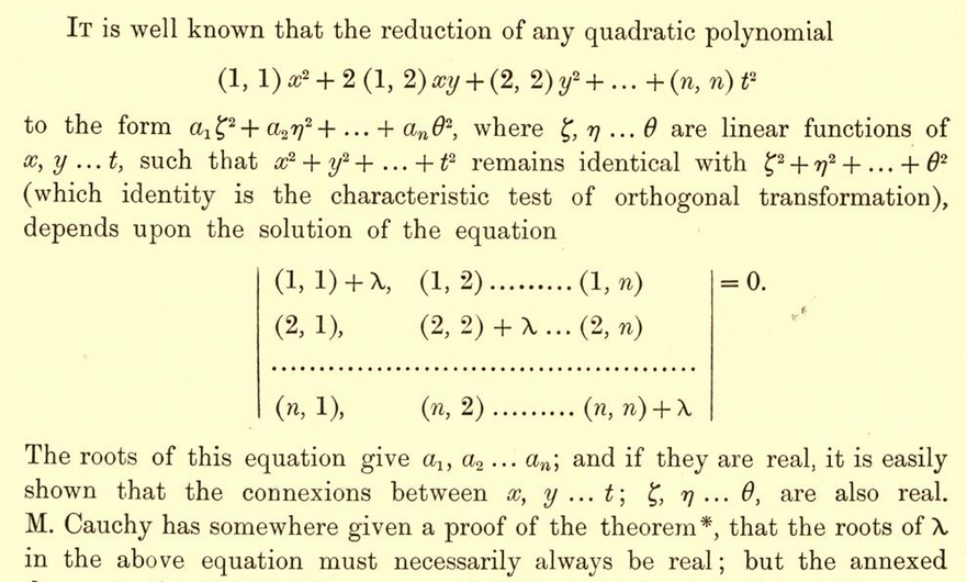
Figure 6. Sylvester's version of Cauchy's eigenvalue problem. From "A Demonstration of the Theorem That Every Homogeneous Quadratic Polynomial is Reducible By Real Orthogonal Substitutions to the Form of a Sum of Positive and Negative Squares" (1852). Image courtesy of Archive.org.

In a footnote, Sylvester referred to proofs of Cauchy's theorem by C. G. J. Jacobi and C. W. Borchardt, but it appears he did not have access to Cauchy's own work on the subject. Two decades later, in 1883, Sylvester published another note in Philosophical Magazine, "On the Equation to the Secular Inequalities in the Planetary Theory," with the obvious intent being to describe the mathematics of secular perturbation. After 21 years of reflection, Sylvester chose the word "latent" to refer to the roots of his matrix determinant, and began the paper with an explanation of this choice.

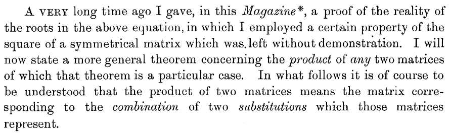
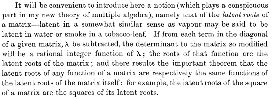
Figure 7. In his paper, "On the Equation to the Secular Inequalities in the Planetary Theory" (1883), Sylvester made the case for naming the latent roots of a matrix. Image courtesy of the University of Michigan Historical Mathematics Collection.

As an aside, we have seen Sylvester's name before in this "Math Origins" series, in his use of the word totient to describe the number of positive integers less than a given integer \(n\) which are relatively prime to \(n\). (He also suggested naming this function with the Greek letter \(\tau\) instead of Gauss's \(\varphi\), but this did not stick.) In both cases, he appeared to have an interest in providing mathematics with clear and rational nomenclature—even if his suggestions were not followed by the mathematical community.

Sylvester's use of "latent" was not the only attempt to rationalize the name of these quantities during this time. In 1896, Henri Poincaré wrote a sprawling, 99-page paper on mathematical equations that often appear in physics. In this paper, "Sur les Équations de la Physique Mathématique" ("On the equations of mathematical physics"), he surveyed the many mathematical equations and techniques that are employed in physics, including a method to solve differential equations which intersects with our interest in eigenvalues. Poincaré began with the differential equation \(\Delta P+\xi P + f D = 0\), where \(\xi\), \(f\), and \(P\) are a scalar, scalar function, and vector field, respectively, and \(\Delta\) denotes the divergence. After considerable analysis of this differential equation, he considered the special case in which \(D\) vanishes.

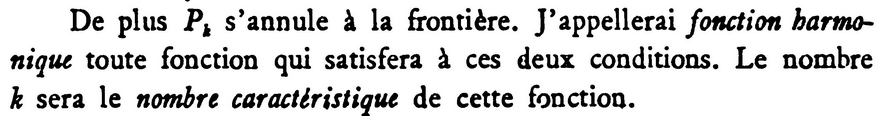
Figure 8. In "Sur les Équations de la Physique Mathématique" (1894), Poincaré chose the terms fonction harmonique and nombre caractéristique for eigenfunctions and eigenvalues. Image courtesy of Archive.org.

As we can see, Poincaré's name for an eigenfunction is "harmonic function," while the name for an eigenvalue is "characteristic number." In a contemporary (but considerably shorter) paper, Émile Picard developed a solution to a second order differential equation. Here, the word "singular" serves to name the eigenvalues, which Picard referred to as "singular points." In the excerpt below, \(y\) is a function of \(x\), \(k\) is a constant, and \(A(x)\) is a continuous, positive function on an interval \((a,b)\).

 

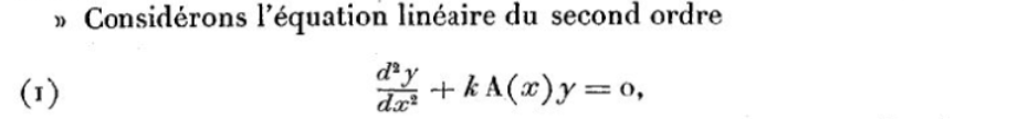
Figure 9. In "Sur les équations linéaires du second ordre renfermant un paramètre arbitraire" (1894), Picard chose the term points singuliers for eigenvalues. Image courtesy of the Bibliothèque Nationale de France's Gallica collection.

We can see that, while Sylvester, Poincaré, and Picard had very different goals in mind, they all felt a need to suggest a name for the roots of their respective equations. So, within the span of about 15 years the words "latent", "singular", and "harmonic" were all added to the mathematician's lexicon. Even though the naming conventions became more muddled during this period, we can at least see that mathematicians had separated the mathematics from the original notion of secular perturbation. Among Sylvester, Poincaré, and Picard, only Sylvester appeared to have a more general exposition in mind—his 1883 paper was meant to advertise a forthcoming work on "multiple algebra," which sought to give a systematic treatment of what would today be called linear algebra. This work is likely to have been "Lectures on the Principles of Universal Algebra," which appeared in Sylvester's American Journal of Mathematics in the following year.

Finding a Proper Eigenwert

So far, we have enjoyed a review of some 19th century works in astronomy and mathematics, and seen the many different names proposed for the solution of a certain matrix determinant calculation—characteristic equations, secular perturbations, singular points, harmonic functions, and latent values have all played a role. The reader may ask at this point: where are the eigenvalues? Indeed, it was not until David Hilbert's 1904 paper "Grundzüge einer allgemeinen Theorie der linearen Integralgleichungen" ("Principles of a general theory of linear integral equations") [Hil1] that our perplexing prefix appeared in print. As the title suggests, this work was meant to provide a general mathematical theory for systems of linear equations, separated (at least in part) from its original context in the theory of celestial mechanics.

Mathematically, Hilbert took real-variable functions \(f(s)\) and \(K(s,t)\) as given, and wanted to find solutions to the equations \[\begin{eqnarray*} f(s) &=& \int_a^b K(s,t)\varphi(t)\,dt \\ f(s) &=& \varphi(s) - \lambda \int_a^b K(s,t)\varphi(t)\,dt\end{eqnarray*}\] where \(\varphi(s)\) and \(\lambda\) represent an unknown function and unknown parameter, respectively. Hilbert called these integral equations of the first kind and second kind, respectively. His goal here was to collect various strands of an idea and consolidate them into a single theory. As he wrote in his introduction,

A closer examination of the subject led me to the realization that a systematic construction of a general theory of linear integral equations is of the greatest importance for all of analysis, especially for the theory of definite integrals and the development of arbitrary functions into infinite series, and also for the theory of linear differential equations, as well as potential theory and the calculus of variations... I intend to reexamine the question of solving integral equations, but above all to look for the context and the general characteristics of the solutions... [Hil1, p. 50].

A careful reading of Hilbert's original text reveals that the word "characteristics" in the above quotation is a translation of the German Eigenschaften, which can mean either "characteristics" or "properties." Here we begin to see the linguistic connection between eigenvalues and Cauchy's équation caractéristique. Soon after, Hilbert described that his method employed "certain excellent functions, which I call eigenfunctions..." While he only claimed to organize and systematize the methods that came before, Hilbert's coinage of "eigenfunction" appears to be new. It is also noteworthy that Hilbert used eigenwerte to refer to eigenvalues.

As the 20th century unfolded, Hilbert's mathematical work heavily influenced the new physical theories of general relativity and quantum mechanics. Two important papers on these subjects are his "Die Grundlagen der Physik" ("Foundations of Physics") [Hil2] and "Über die Grundlagen der Quantenmechanik" ("Foundations of Quantum Mechanics") [HNN], which appeared in Mathematische Annalen in 1924 and 1928, respectively. The eigen- prefix appears in both papers. In the former, Hilbert coined the word Eigenzeit (in English, "eigentime") for eigenvalues of a particular matrix, while in the latter, he used both Eigenwert and Eigenfunktion when analyzing the Schrödinger wave equation. One of Hilbert's coauthors on this latter paper was a young John von Neumann, who emigrated to the United States in 1933 and made lasting contributions to both mathematics and physics. Crucially, von Neumann's long residence in the United States (he became a citizen in 1937) made his work more influential than most when it came to the choice of mathematical terminology. Now publishing mostly in English, von Neumann translated Hilbert's eigenfunktion as proper function (for an example, see [BvN]). While this usage was picked up by von Neumann's students and acolytes in North America, the half-translated form (eigenvalue for eigenwert, etc.) remained popular as well.

Conclusion

By the middle of the 20th century, there were at least five different adjectives that could be used to refer to the solutions in our particular type of matrix equation: secular, characteristic, latent, eigen, and proper. In general, though, two naming conventions dominated: eigen- (from Hilbert's German writings) and characteristic/proper (from Cauchy's French writings and von Neumann's translation of eigen-). In the United States, the peculiar prefix eigen- won the debate, as described amusingly by Paul Halmos in his introduction to A Hilbert Space Problem Book in 1967:

For many years I have battled for proper values, and against the one and a half times translated German-English hybrid that is often used to refer to them. I have now become convinced that the war is over, and eigenvalues have won it; in this book I use them." [Hal, p. x]

By the time this book appeared in 1967, Halmos clearly felt the debate was over in the United States. While this is true, the global battle is not over! Both naming conventions are still in use around the world. A cursory search of modern languages reveals that mathematicians are still split on the issue. With apologies to those with more language expertise than I, here is a rough accounting of the word for "eigenvalue" in several widely-spoken languages around the world.

Language	Word(s) for "eigenvalue"	Literal translation
Arabic	القيمة الذاتية	self-value
German	Eigenwert	self-value
Russian	собственное значение	self-value
Chinese	特征值	characteristic value
French	valeur propre	proper value
Portuguese	valor propio, autovalor	proper value, self-value
Spanish	valor próprio, autovalor	proper value, self-value

As you can see, translations of Hilbert's eigen- prefix hold sway in Arabic, German, and Russian, while proper has taken hold in French, Portuguese, and Spanish. Of course, there is some ambiguity here, in that Portuguese and Spanish have words for both versions, and the Chinese text does not translate cleanly into either version. Note though, the English language's use of an untranslated German prefix—all other languages appear to translate from German or French using a word meaning "intrinsic" or "self" or "proper." So the peculiar prefix eigen- is not so peculiar after all. Rather, the peculiarity is that English uses a German prefix without translating it.

References

[BvN] Birkhoff, Garret and von Neumann, John. "The Logic of Quantum Mechanics," Annals of Mathematics, Second Series, 37 No. 4 (Oct. 1936), 823-843.

[Cau1] Cauchy, A.-L. "Sur l'équation à l'aide de laquelle on détermine les inégalités séculaires des mouvements des planétes," Exercises de mathématiques 4, in Œuvres complètes d'Augustin Cauchy, Paris: Gauthier-Villars et fils, 2 No. 9, 174-95.

[Cau2] Cauchy, A.-L. "Mémoire sur l'integration des équations linéaires," Exercises d'analyse et de physique mathématique, 1 (1840), 53-100.

[Hal] Halmos, Paul R. A Hilbert Space Problem Book. Princeton, NJ: D. Van Nostrand Company, Inc., 1967.

[Haw1] Hawkins, T. W. "Cauchy and the spectral theory of matrices," Historia Mathematica, 2 (1975), 1-29.

[Hil1] Hilbert, David. "Grundzüge einer allgemeinen Theorie der linearen Integralgleichungen," Nachrichten von d. Königl. Ges. d. Wissensch. zu Göttingen (Math.-physik. Kl.), (1904), 49-91.

[Hil2] Hilbert, David. "Die Grundlagen der Physik," Math. Annalen, 92 Issue 1-2 (March 1924), 1-32.

[HNN] Hilbert, David, von Neumann, John, and Nordheim, Lothar. "Über die Grundlagen der Quantenmechanik," Math. Annalen, 98 Issue 1 (March 1928), 1-30.

[Pic] Picard, Émile. "Sur les équations linéaires du second ordre renfermant un paramètre arbitraire," Comptes Rendus Hebdomadaires Séances de l'Académie des Sciences, 118 (1894), 379-383.

[Poi] Poincaré, Henri. "Sur les Équations de la Physique Mathématique," Rendiconti del Circolo Matematico di Palermo, 8 (1894), 57-155.

[Syl1] Sylvester, J. J. "A Demonstration of the Theorem That Every Homogeneous Quadratic Polynomial is Reducible By Real Orthogonal Substitutions to the Form of a Sum of Positive and Negative Squares," Philosophical Magazine, 4 (1852), 138-142.

[Syl2] Sylvester, J. J. "On the Equation to the Secular Inequalities in the Planetary Theory," Philosophical Magazine, 16 (1883), 267-269.

 

Once a mathematics student becomes proficient in the mathematical calculations of the calculus and statistics, there is often a moment when the logical superstructure of mathematics becomes apparent. This may manifest itself through explicit questions, or at least some discomfort about the supposed reliability of mathematical truths. How can we be sure that classic results such as the mean value theorem or the central limit theorem are true? What about the existence of the real numbers themselves? This is the point at which many undergraduate mathematics curricula include a course on mathematical logic and thought.

In the author's own experience, this typically involves a reversal of the order of ideas, from the "order of discovery" so common in problem-solving to the "order of logic" that forms the underlying foundation for mathematical proofs. It becomes clear very quickly that new terms and notations are required to elucidate the mathematical statements and logical relationships at play. Notions such as conjunction and disjunction, implication and equivalence, the universal and the existential, must be carefully separated from one another. Today, the theory of logic and its corresponding notation are viewed as a package: one does not exist independently of the other. However, this was not always so! In this article, we explore some early attempts to organize the theory of logic in systematic ways, along with some of the notational choices that were made. We will find that authors of the 17th and 18th centuries were primarily interested in describing a way of thinking about logic, usually by analogy with pre-existing mathematical or philosophical concepts. In the next article in this series, we will advance the narrative into the 19th and 20th centuries to examine the multitude of notational systems that were proposed for logic.

Some Early Symbols from Johann Rahn

For many students, some logic symbols appear early in their mathematical learning, often as a shortcut or abbreviation to simplify one's thought process. A good example of this is the \(\therefore\) symbol for "therefore," used to conclude a chain of reasoning. An early adopter of this symbol was the Swiss mathematician Johann Rahn. In his 1659 book, Teutsche Algebra (German Algebra) [Rah], Rahn sought to relate the algebraic contributions of Viète, Descartes, and others to a German-language audience. In doing so, he used a number of notational shortcuts to express those ideas. Here's an excerpt.

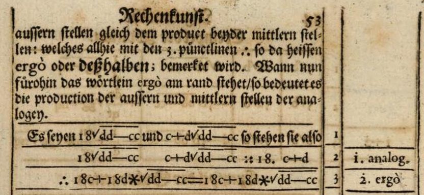
Figure 1. An algebraic argument in Johann Rahn's Teutsche Algebra (1659) uses \(\therefore\) for "therefore" and * for multiplication. Digitized by Google Books from the copy owned by the Bavarian State Library.

In the second line of this passage, Rahn defined the "three points \(\therefore\)" symbol to carry the same meaning as the Latin ergo. This symbol appears at the conclusion of the argument immediately following: the proportion \(18\sqrt{dd-cc} : (c+d)\sqrt{dd-cc} :: 18 : c+d\) from step 2 is resolved in step 3 as the tautological equation \((18c+18d)\cdot\sqrt{dd-cc} = (18c+18d)\sqrt{dd-cc}\). (Today we would describe this step as using cross-multiplication and distribution to solve a fraction problem.) According to Cajori [Caj, p. 212], this was the first use of \(\therefore\) to mean "therefore." We should also note the column on the right-hand side, in which he referred back to previous steps along with an abbreviated description of the logic for the given step.

Rahn's notational contributions did not end here; 20 pages later he used a few novel symbols to elucidate the logic of a familiar algebraic argument.

Figure 2. Some interesting logic symbols from Johann Rahn's Teutsche Algebra (1659). Digitized by Google Books from the copy owned by the Bavarian State Library.

In this extract, Rahn gave an approach to solve an old problem: given numbers \(D\) and \(F\), find numbers \(a\) and \(b\) whose sum and product equal \(D\) and \(F\), respectively. Rahn has introduced a spiral symbol for exponentiation in line 3, an asterisk * for multiplication in line 4, and what can only be described as a "squiggle" for the square root in line 6. At the end, he has found an expression for \(a-b\) which may then be added to or subtracted from \(a+b = D\), thus replicating the quadratic formula. As used here, these new symbols are a notational shortcut to organize the logic of an argument, not too different from two-column proofs that are used by today's students to organize mathematical proofs.

Leibniz's Pursuit of a Universal Mathematics

In one sense, Rahn merely introduced some symbols to streamline existing arguments, rather than to think systematically about how arguments were constructed. (To be fair to Rahn, this was a valuable innovation in an era when the expense of paper and printing was a nontrivial consideration.) Indeed, it was not for another generation that an attempt was made to systematize logic, by none other than Gottfried Wilhelm Leibniz. For a philosophically-minded scholar as Leibniz, this was part of a more ambitious project: a symbolic and rigorous universal calculus that could be applied to any project in the realm of human inquiry. This was a research program that Leibniz pursued in various forms throughout his long career. As described by Garrett Thomson in his small volume, On Leibniz [Tho, p. 15 ff.], Leibniz had three major goals:

1. Create an alphabet of logic, in which concepts may be encoded in numerical form;

2. Create a dictionary of logic, so that complex concepts may be translated into numerical language;

3. Create a syntax of logic, to govern the ways in which inferences may be made.

The first goal appeared in Leibniz's writing as early as 1666, in the treatise Dissertatio de Arte Combinatoria (Dissertation on the Art of Combinations) [Lei]. Specifically, Leibniz asserted that all propositions (1) can be stated in subject-predicate form, and (2) can be constructed as "complexions" (or, combinations) of simple propositions. In counting the number of ways these complexions can be made from a set of simple propositions, Leibniz was led to the Pascal triangle from combinatorics.

Interestingly, this early treatise on logic was the only such work published by Leibniz during his lifetime. However, Leibniz did devote considerable time to his overall project, ultimately writing over a dozen treatises on various topics in logic. The year 1679 was apparently a fruitful time for Leibniz, as he wrote six papers on the universal calculus that spring. We will explore one of these six, the ambitiously-titled "Regulae ex quibus de bonitate consequentiarum formisque et modis syllogismorum categoricorum judicari potest, per numeros" ("Rules from which a decision can be made, by means of numbers, about the validity of inferences and about the forms and moods of categorical syllogisms"). In his first example, Leibniz deconstructed the proposition "Every wise man is pious" in the following way:

A true universal affirmative proposition, for example

Every wise man is pious 

\(+20\;\;\;\;\;\;-33\;\;\;\;\;\;+10\;\;\;\;\;\;-3\)

\(+cdh\;\;\;\;\;\;-ef\;\;\;\;\;\;+cd\;\;\;\;\;\;-e\)

is one in which any symbolic number of the subject (e.g. \(+20\) and \(-33\)) can be divided exactly (i.e. in such a way that no remainder is left) by the symbolic number of the same sign belonging to the predicate (\(+20\) by \(+10\), \(-33\) by \(-3\)). So, if you divide \(+20\) by \(+10\) you get \(2\), with no remainder, and if you divide \(-33\) by \(-3\) you get \(11\), with no remainder. Conversely, when this does not hold the proposition is false. [Par, p. 26]

There are three important observations to make here. First, Leibniz was careful to distinguish between subject and predicate in his statements. Indeed, at the outset of the paper he remarked that "every categorical proposition has a subject, a predicate, a copula; a quality and a quantity." In the above example, the subject "wise man" and predicate "pious" are related via the copula "is", and quality of the proposition is "affirmative." According to Thomson [Tho, p. 20], the subject-predicate relationship was one of Leibniz's fundamental assumptions about logic. Second, Leibniz also distinguished between universal and particular statements. Today, we would refer to universally-quantified and existentially-quantified statements. This increases the level of precision possible when formulating propositions. Lastly, both of these previous facts allowed for a statement to be encoded in terms of integer divisibility. Specifically, the predicate will "divide evenly" into the subject exactly when the proposition is true.

A Wider View: Richeri's Algebrae Philosophicae

Fast forward to 1761, when Ludovico Richeri's Algebrae philosophicae in usum artis inveniendi (An algebra of philosophy, for use in the art of discovery) appeared in print. As the title suggests, Richeri introduced a set of notations to better express logical ideas.

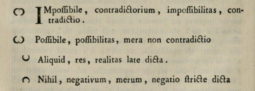
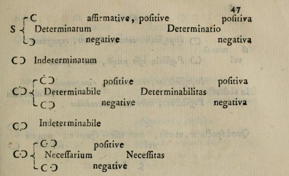
Figure 3. Richeri's set of symbols for representing logical ideas in the Algebrae philosophicae (1761). Digitized by Archive.org from the copy owned by the Natural History Museum Library, London.

As we can see, two circle arcs are used in varying combination to represent logical ideas. For example, the symbol resembling the Greek letter \(\omega\) is used for statements that are deemed possible, while an inverted version of this symbol \(\mho\) is used for contradictory statements. The text continues with an extensive list of symbol pairs that express contrasting concepts in logic: thing and nothing, positive and negative determinations, determinate and indeterminate, possibility and impossibility, mutable and immutable. Most importantly, Richeri's symbols for thing (aliquid) and nothing (nihil) resemble today's symbols for union (\(\cup\)) and intersection (\(\cap\)), respectively. This climax of this short article is a logic diagram that traces the possible outcomes of any object of critical inquiry.

Figure 4. Richeri's tree of logic symbols from the Algebrae philosophicae (1761). Digitized by Archive.org from the copy owned by the Natural History Museum Library, London.

In purely symbolic form, Richeri has given a sort of binary search for philosophical inquiry—indeed, this is the algebraic philosophy that was promised! In words, the tree begins like this:

• Any statement is either impossible (contradictory, the inverted \(\omega\) in the corner) or possible (noncontradictory, the \(\omega\) at the left end of the tree);

• If a statement is possible (\(\omega\)), it is either determinate (proven, the lower branch) or indeterminate (unproven, the upper branch);

Following the tree a bit further, we see that any possible, determinate statement must be either affirmative or negative. It's also interesting that Richeri viewed possible, indeterminate statements as being either determinable (provable) or indeterminable (unprovable). All told, Richeri's Algebrae philosophicae is only 16 pages long, with many of those consisting of symbolic representations for various propositions. If you have detected echoes of Leibniz in this paper, you are correct! This is no accident: Richeri specifically cited the Dissertatio de Arte Combinatoria in his work. Specifically, we can see how the subject-predicate form of a proposition has been carried over into the Algebrae philosophicae.

Lambert's Zeichenkunst in der Vernunftlehre

Not long after Richeri's algebra of philosophy was published, Johann Lambert made his own attempt at a symbology of reason in his 1782 work, Sechs Versuche einer Zeichenkunst in der Vernunftlehre (Six attempts at a drawing-art in the theory of reason) [Lam]. Here are Lambert's symbols, from page 5.

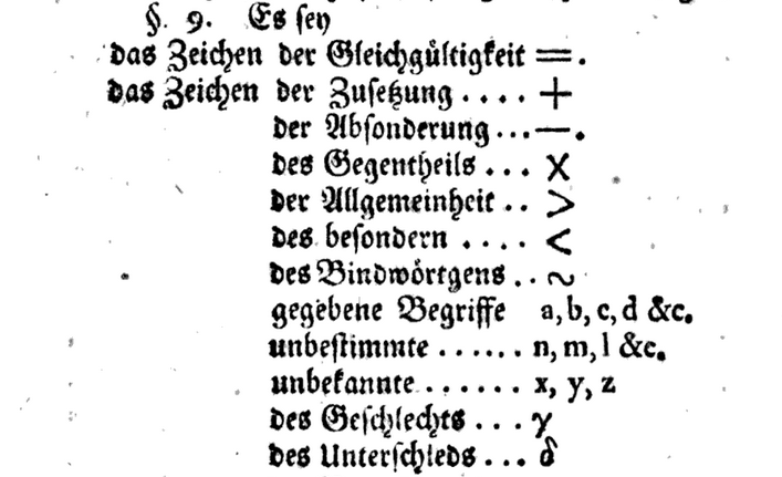
Figure 5. Johann Lambert appropriated symbols from algebra and arithmetic to represent logical ideas in Sechs Versuche einer Zeichenkunst in der Vernunftlehre (1782). Digitized by Google Books from the copy owned by the Bavarian State Library.

We see here that Lambert's symbols are more mathematical and less philosophical than Richeri's. In addition to appropriating symbols from mathematics, their meanings are easily recognizable to any modern student of logic; for instance, note the signs for equality (\(=\)), addition (\(+\)), separation (\(-\)), opposition (\(\times\)), universality (\(>\)), and particularity (\(<\)). The idea here seems to be that all analysis of logical ideas should and can be reduced to a form of arithmetic. In this sense, Lambert's approach is much closer to Leibniz, since it relies on an analogy between logic and arithmetic. (Also notice that all three men distinguished between the universal and the particular.)

To see Lambert's arithmetic approach in action, let's consider one of his earlier examples [Lam, p. 11]. Given two statements \(a\) and \(b\), Lambert used \(ab\) to denote that which they had in common, so consequently \(a-ab\) represents those characteristics of \(a\) that are not possessed by \(b\). Interestingly, Lambert's phrase for this is "eigene Merkmale," which could be reasonably translated as "self-characteristics," an echo of the eigen- prefix from an earlier article in this series. By the same token, \(b-ab\) represents those characteristics of \(b\) that are not possessed by \(a\). Thus, the expression \(a+b-ab-ab\) refers to the self-characteristics of \(a\) and \(b\) taken together, today known as a symmetric difference. For this to work, notice that Lambert's \(+\) must be construed not as a union, but as a combination (with possible repetition) of \(a\) and \(b\). At any rate, this concept was given its own symbol, so that \(a\mid b\) represents the aspects of \(a\) that are not shared with \(b\), and vice versa. This results in the logic equation \(a\mid b + b\mid a + ab + ab = a+b\), which states that combining the self-characteristics of \(a\) and \(b\) with two copies of their intersections yields the same result as combining \(a\) and \(b\).

Conclusion... For Now

As we have seen, the general struggle during this period was to develop a way of thinking about logic. Leibniz had a vision—however incomplete—of a universal calculus based on subject-predicate language, Richeri used a philosophy-infused approach to classify statements and provability, and Lambert introduced a notational system to represent logical ideas. The first and last of these relied on an analogy with arithmetic, in that statements and inferences were represented by numbers and operations, respectively. Lambert's method in particular seems like an early Venn diagram in symbolic form, though he thought of his objects as unities possessing several qualities, rather than as sets possessing several elements.

Not surprisingly, this story is hardly over! Some 60 years after Lambert's attempt at systematizing logic, Augustus De Morgan wrote his Formal Logic (subtitled more descriptively as The Calculus of Inference) with much the same goals as his predecessors. In this 1847 publication, De Morgan cleared up at least some of the confusion by formalizing Leibniz's notions of universal and particular through introducing quantification into his calculus. Here is one glimpse of his writing on this subject, in which the word quantity is used to make the distinction between universal and particular.

Figure 6. Augustus De Morgan's explanation of converse forms in mathematical logic, from Formal Logic (1847). Digitized by Archive.org from the copy owned by the University of Toronto Library.

For now, note that some other glimpses from this book can be found on Convergence as one of Frank Swetz's Mathematical Treasures. In the sequel, we will pick up the story with a deeper examination of De Morgan's work in Formal Logic, with a special interest in the notation he chose for quantification. Then we will examine how the struggle of the 19th and 20th centuries was to develop a way of writing about logic. Ultimately, the rise of set theory was to have a profound impact on mathematical logic, and it led to a corresponding change in notations. More on this next time!

References

[Caj] Cajori, Florian. A History of Mathematical Notations, Volume II. Chicago: Open Court Publishing Co., 1928.

[DeM] De Morgan, Augustus. Formal Logic: or, the Calculus of Inference, Necessary and Probable. London: Taylor and Walton, 1847.

[Lam] Lambert, Johann. Sechs Versuche einer Zeichenkunst in der Vernunftlehre. Berlin, 1782.

[Lei] Leibniz, Gottfried Wilhelm, Dissertatio de arte combinatoria. Leipzig, 1666. Available in English translation in Philosophical Papers and Letters (Leroy E. Loemker, editor, 2nd edition) from 1969. Two images are provided in Mathematical Treasures.

[Par] Parkinson, G. H. R., ed. Leibniz Logical Papers. Oxford: Clarendon Press, 1966. Contains many English translations of Leibniz's unpublished works.

[Rah] Rahn, Johann. Teutsche Algebra. Zurich: J. J. Bodmer, 1659.

[Ric] Richeri, Ludovico. "Algebrae philosophicae in usum artis inveniendi." Melanges de philosophie et de la mathématique de la société royale de Turin 1 (1760-61), 46-63.

[Tho] Thomson, Garrett. On Leibniz. Stamford, CT: Thomson Learning, 2001.

 

In our last article, we explored the struggles of 17th- and 18th-century mathematicians who sought to devise a coherent system for describing logical ideas, and a few novel attempts at establishing a system of symbols to express those ideas. Contributions ranged from Gottfried Wilhelm Leibniz's vision of a "universal calculus" that could encode any logical statement with mathematical precision to Ludovico Richeri's binary-tree system for classifying logical statements in terms of their philosophical qualities.

By the early 19th century, then, mathematicians possessed a number of different methods for representing logical statements, including Leibniz's numerical system and Johann Lambert's appropriation of arithmetic symbols in Sechs Versuche einer Zeichenkunst in der Vernunftlehre (Six attempts at a drawing-art in the theory of reason). In this article, we continue the narrative through the 19th and 20th centuries, during which time the logical ideas of past centuries were tamed: not only through a symbol system, but also through a system for manipulating them. Eventually, the familiar symbols of today's mathematical logic emerged, alongside the terminologies typically used to describe them.

The British Duo: Boole and De Morgan

With the start of the 19th century, our narrative shifts from the European continent to Britain, where Augustus De Morgan and George Boole were to make lasting contributions to logic and (eventually) computer science. In fact, the two men maintained a long-term correspondence with each other, beginning in 1842. As we will see, however, their approaches to the study of logic were quite different.

Born in India to British parents, De Morgan returned to Britain as an infant, later joining Trinity College at Cambridge University at age 16. Remarkably, at the age of 22 he found himself appointed chair of mathematics at London University (now University College London). While not directly connected to our goals for this article, this happens to be the time at which De Morgan provided a modern definition (see [DeM1]) of the method of proof that we today call "mathematical induction," as part of a series of articles for the Penny Cyclopedia. Until then, the word "induction" was often used to refer to what today's mathematicians would call "proof by example"—an erroneous method of proving mathematical truth that relies on an observed pattern.

In the decades following his 1828 appointment to London University, De Morgan's interest in logic continued, culminating with his publication of Formal Logic: or, The Calculus of Inference, Necessary and Probable, in 1847. De Morgan's book advertised a "simple notation" to express any proposition by using only three letters, and a "subordinate notation" to abbreviate it. Chapter 1, titled "First Notions," begins with a discourse on propositions, which are described as a subject and predicate linked by a copula. Properly quantified, there are four species of proposition in De Morgan's telling.

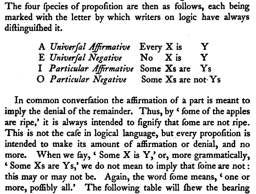
Figure 1. De Morgan's presentation of the quantified logic statements denoted by the vowels \(A\), \(E\), \(I\), \(O\) in Formal Logic (1847). Image courtesy of Archive.org [DeM2].

Using the language of set theory, we may translate De Morgan's vowels \(A\), \(E\), \(I\), \(O\) in the following way:

• \(A\):  For all \(x\in X\), it follows that \(x\in Y\).
• \(E\):  For all \(x\in X\), it follows that \(x\not\in Y\).
• \(I\):  There exists \(x\in X\) for which \(x\in Y\).
• \(O\):  There exists \(x\in X\) for which \(x\not\in Y\).

Aside from the fact that De Morgan used the word "particular" in place of "existential," the classification system is essentially the same as in any logic textbook today. In fact, the entire chapter is a pleasant tour of the fundamental concepts in predicate calculus, with many familiar concepts wearing nearly the same clothing as today—the interested reader is highly encouraged to read it for its own sake! For our purposes, we move to Chapter 4, "On Propositions," in which De Morgan introduced his system for expressing propositions symbolically. On page 60, we find the following notations to write these quantified statements in a fully symbolic form:

• \(X)Y\) – "Every \(X\) is \(Y\),"
• \(X.Y\) – "No \(X\) is \(Y\),"
• \(X:Y\) – "Some \(X\)s are not \(Y\)s,"
• \(XY\) – "Some \(X\)s are \(Y\)s."

This new notational system allowed De Morgan to characterize the six distinct "modes" of proposition that can be built from \(X\) and \(Y\):

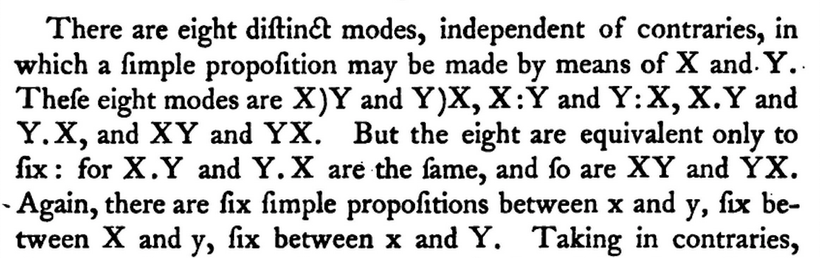
Figure 2. De Morgan's six "modes" of proposition formed from simple propositions \(X\) and \(Y\), from Formal Logic (1847). Image courtesy of Archive.org.

In his notation, \(x\) and \(y\) are the negations of \(X\) and \(Y\). Since each pair of letters may be combined into six distinct simple propositions, there are at most \({4\choose 2}\cdot 6 = 6\cdot 6 = 36\) possible modes. De Morgan did not consider contradictory statements such as \(X)x\) or tautologies such as \(y:Y\), so he only counted 24 possible modes. A little thought reduces the list to eight distinct propositions:

Figure 3. In Formal Logic (1847), De Morgan noted eight distinct modes of proposition based on the simple propositions \(X\) and \(Y\) and their negations \(x\) and \(y\). Image courtesy of Archive.org.

In De Morgan's system, then, any of eight distinct modes of expression may be referred to with one of \(A\), \(E\), \(I\), \(O\), and an accompanying superscript or subscript mark. While the notation obscures the underlying logical concepts (for example, the letters \(A\) and \(E\) give no indication that their referents are both universally-quantified statements), it is certainly comprehensive, providing a self-contained system for writing statements logically.

In the same year that De Morgan's Formal Logic appeared in print, George Boole made the first of several contributions to logic with The Mathematical Analysis of Logic, Being an Essay Towards a Calculus of Deductive Reasoning [Boo1]. In fact, as the logician Clarence Lewis related in A Survey of Symbolic Logic (1918), Boole and De Morgan's works were published on the very same day in 1847. Along with Lewis, we observe that Boole's approach to logic "allows operations which have no direct logical interpretation, and is obviously more at home in mathematics than in logic. It is probably the great advantage of Boole's work that he either neglected or was ignorant of these refinements of logical theory which hampered his predecessors" [Lew, p. 51].

Unlike De Morgan, Boole had difficulty obtaining a university appointment. This was due in part to the fact that he was largely self-educated in mathematics. He was eventually appointed, in 1849, to Queen's College, Cork. In 1854 he produced a second, more comprehensive work on logic titled An Investigation of the Laws of Thought on Which are Founded the Mathematical Theories of Logic and Probabilities [Boo2]. As a youth, Boole had demonstrated an early propensity for language, having taught himself Greek, French, and German. Unsurprisingly for one with Boole's background in languages, he began Chapter 2 of his Laws of Thought with a definition of a "sign":

Figure 4. Boole began his Laws of Thought (1854) by reflecting on the denotative meaning of written language and giving a definition of a sign. Image courtesy of Archive.org.

In Boole's view, any mark with a fixed interpretation counts as a "sign," and—crucially—the laws for manipulating signs are independent of any particular symbol system. This frees the logician to choose among any existing symbols (or create new symbols) to describe logical ideas. Naturally enough, Boole's first proposition establishes one way to reappropriate the symbols and rules of algebra for use in mathematical logic:

Figure 5. Boole's catalog of symbols from Laws of Thought (1854). Image courtesy of Archive.org.

In this way, Boole may give a more granular accounting of the ideas in logic, more like an "atomic" form of reasoning, when compared to De Morgan's approach in Formal Logic. Moreover, while his symbolic choices were similar to Lambert's approach from the previous article, Boole's overall framework is more systematic than that of Lambert. In particular, Boole chose to reserve different types of symbols to refer to "subjects" and others to refer to "operations of the mind." For an example, let us skip ahead to page 33:

Figure 6. An example of Boole's symbol system in use, from Laws of Thought (1854). Image courtesy of Archive.org.

Here, \(x\), \(y\), and \(z\) are subjects of our conception, while addition and multiplication are operations of the mind. This allows Boole to conceive of the phrase "European men and women" as being identical to "European men and European women." (As an aside: mathematics was not Boole's only interest in this work; take a look at this selection from Boole in the Mathematical Treasures series in which he gives a proof of the existence of a Aristotelian-style "prime mover.")

Boole was to exert a heavy influence on the next several decades of research in logic, including with a young Ernst Schröder, who wrote in 1877 that, in logic, "it is now possible to obtain the utmost attainable simplicity and perfection—a goal whose realization, after Boole's preliminary work, requires only fairly straightforward observations" [Sch1, p. IV]. In this work, Der Operationskreis des Logikkalkuls, Schröder developed a Boolean-style system for the calculus of logic, observing that "Nothing prevents naming those 4 basic [arithmetic] operations with the same names and expressing them with the same symbols as are used in arithmetic. After all, the object of the operations is a completely different one—there they are numbers, but here they are arbitrary concepts!" [Sch1, p. 2]. This may seem an unnecessary observation to a modern reader, but this is likely because of Boole's influence rather than in spite of it. We now turn to the intellectual descendants of both Boole and De Morgan as the 19th century reached its conclusion.

The Lightning Round: Symbol Systems from the late 1800s

The number of works in logic increased greatly during the late 19th century, so here we will take a brief tour of a few notable works and symbol choices from this period. First, we take a peek at Schröder's Vorlesungen über die Algebra der Logik (Lectures on the Algebra of Logic), which appeared in 1890. Notably, it introduces the \(\subset\) symbol to indicate "subordination," which Schröder compared to the \(<\) symbol used with numbers.

Figure 7. Ernst Schröder's introduction of the \(\subset\) symbol in Vorlesungen über die Algebra der Logik (Lectures on the Algebra of Logic),  published in 1890 [Sch2, p. 129]. Image courtesy of Göttingen State and University Library.

While the \(\subset\) symbol is used today to denote the containment of sets, Schröder's intent was more general—the containment can refer to the content of either sets or logical ideas. Interestingly, Schröder overlaid an \(=\) over the \(\subset\) to indicate the "subordinate or equal to" relationship, in contrast to today's \(\subseteq\) symbol.

Figure 8. Ernst Schröder's use of \(\subset\) and  \(\subset\!\!\!\!\!=\) symbols in Vorlesungen über die Algebra der Logik (Lectures on the Algebra of Logic), published in 1890 [Sch2, p. 132]. Image courtesy of Göttingen State and University Library.

At the end of this passage, the "subordinate or equal to" symbol is used as a way to show how the subject of a proposition is either "contained in" or "equivalent to" the predicate. On page 130, we find an appraisal of some alternative symbols in use at the time, including Paul Du Bois-Reymond's \(\prec\) (seen in a previous article in this series) and C. S. Peirce's \(-\!\!\!<\). Peirce, an American mathematician, was a founder of the pragmatist school of philosophy and made significant contributions to logic throughout the late 19th century. Familiar with the work of De Morgan and Boole, a young Peirce published "On an Improvement in Boole's Calculus of Logic" in the 1868 Proceedings of the American Academy of Arts and Sciences. In this short paper—appearing some 20 years before Schröder's Vorlesungen über die Algebra der Logik—Peirce proposed that Boole's symbol usage from Laws of Thought be adapted by placing a comma atop the various arithmetic symbols used for logical analysis.

Figure 9. C. S. Peirce used a comma to indicate when the symbols of arithmetic were used to denote logical concepts. From his 1868 work, "On an Improvement in Boole's Calculus of Logic" [Pei, p. 402]. Image courtesy of Biodiversity Heritage Library.

Having established his alternative symbol system, Peirce then laid out a set of familiar theorems in his new system, including reflexivity (Theorem I) and transitivity (Theorem II).

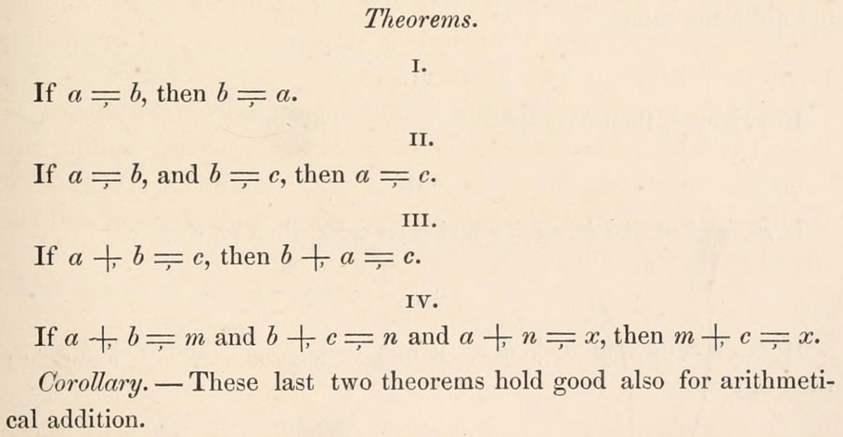
Figure 10. Peirce's first set of theorems using his comma notation. From his 1868 work, "On an Improvement in Boole's Calculus of Logic" [Pei, p. 403]. Image courtesy of Biodiversity Heritage Library.

In later years, Peirce's interests grew to include astronomy, the philosophy of science, and statistics. As a philosopher, he became attracted to symbols in a more abstract sense, developing a three-category system to describe them. In The Math Gene [Dev], Keith Devlin describes the three categories as icon, index, and symbol. The last of these sits at the apex of this mental edifice; in Devlin's words,

An object, action, event, or entity X is called a symbol for some other object, action, event, or entity Y if there is an agreed convention whereby X represents (or symbolizes) Y, irrespective of the physical nature of X and Y. For example, a wedding ring is symbolic of the fact that the wearer is married. Nothing about a band of gold worn around the third finger of the left hand intrinsically represents a married state. The meaning is purely by convention [Dev, p. 208].

In Peirce's view, all human language is symbolic—words themselves have meaning only via the consensus of those who speak them. This takes us beyond the scope of this article, though it should be clear how Boole's use of the "sign" in logic lurks in the background of Peirce's philosophy of "symbol".

We choose to end the century in 1901, with Giuseppe Peano's Formulaire de Mathématiques (The Form of Mathematics). Peano adopted Boole's convention of using letters to represent "objects of the mind" and Schröder's \(\subset\) for logical containment, while also distinguishing between propositions (statements which are either true or false) and classes (collections of instances) in his notational system. Especially note the use of \(x\varepsilon a\) in Rule 4 to denote that \(x\) is an instance of the class \(a\).

Figure 11. Giuseppe Peano's 1901 definition of "classes" in Formulaire de Mathématiques [Pea, p. 1]. Image courtesy of Archive.org.

Rule 7 illustrates the form taken in Peano's logic: "Given classes \(a\) and \(b\), \(a\supset b\) means 'every \(a\) is \(b\).' Given propositions \(p\) and \(q\) which contain a variable \(x\); [we write] \(p.\supset x.q\) to mean 'from \(p\) we deduce, regardless of \(x\), that \(q\) [is true]'." While the universal quantification is not spelled out in the notation, we have here a nice melding of Boole's conventions with Schröder's notion of logical containment.

While this ends the lightning round, we note that there are many valuable teaching resources on the history of logic that expand on these authors' contributions, including Jerry Lodder's Deduction through the Ages: A History of Truth (2013), published in Convergence. In particular, interested readers can learn more about the work of Boole, Venn, and Peirce in Origins of Boolean Algebra in the Logic of Classes (2013) by Janet Barnett, also published in Convergence.

Epilogue: The Principia Mathematica

Around the time Peano was working on Formulaire de Mathématiques, he attended the International Congress of Philosophy in 1900, where he met a young Bertrand Russell. Writing in his autobiography many years later, Russell recalled this meeting:

I already knew [Peano] by name and had seen some of his work, but had not taken the trouble to master his notation. In discussions at the Congress I observed that he was always more precise than anyone else, and that he invariably got the better of any argument on which he embarked. As the days went by, I decided that this must be owing to his mathematical logic. ... It became clear to me that his notation afforded an instrument of logical analysis such as I had been seeking for years... [Rus, p. 144].

A decade later, Russell and Alfred North Whitehead produced the Principia Mathematica, an ambitious work published in three volumes from 1910 to 1913. In it, Russell and Whitehead sought to give a systematic and rigorous accounting of mathematical truths using symbolic logic. As Russell wrote in the introduction to the second edition in 1963, the Principia was "framed with a view to the perfectly precise expression, in its symbols, of mathematical propositions" [WR, p. 1]. As one would expect, a goal as lofty as this one required a notational system equal to the task. This is the task of Chapter 1, which the authors begin by observing their debt to Peano: "The notation adopted in the present work is based upon that of Peano, and the following explanations are to some extent modelled on those which he prefixes to his Formulario Mathematico." The notational choices are spread throughout this chapter, but we list some of them here (all page numbers correspond to the second edition of Volume I):

• Page 6: "The Contradictory Function with argument \(p\) ... is denoted by \(\sim p\)."

• Page 6: "The Logical Sum ... is denoted by \(p\lor q\)."

• Page 6: "The Logical Product ... is denoted by \(p.q\), or—to make the dots act as brackets in a way to be explained immediately—by \(p:q\), or by \(p:.q\), or by \(p::q\)."

• Page 7: The equivalence of two statements \(p\) and \(q\) is "denoted by \(p\equiv q\)."

• Page 8: "The sign '\(\vdash\),' called the 'assertion sign,' means that what follows is asserted." (This was borrowed from Gottlob Frege.)

This is neatly summarized on page 12:

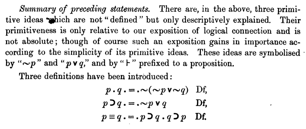
Figure 12. Whitehead and Russell's summary of the basic concepts and symbols in their propositional calculus. From Volume I of Principia Mathematica (1910). Image courtesy of HathiTrust Digital Library.

In this way, Whitehead and Russell gave three descriptive concepts (negation, disjunction, and assertion) and three rigorously-defined concepts (conjunction, implication, and equivalence), each with their own symbolic shorthand. Continuing further into the work, we find the symbol \(\exists\) used for existentially-quantified statements, and De Morgan's notation \(p)q\) borrowed occasionally to denote implications. There is much more in this work, so perhaps the best suggestion is for readers to explore it for themselves, either by browsing this Mathematical Treasure or paging through the second edition of Volume I on Archive.org.

Much more could be said of Whitehead and Russell's work, not to mention the many contributors whose works were left out of this survey. For now, we conclude with an observation from Florian Cajori, whose A History of Mathematical Notations formed the backbone of this article:

No topic which we have discussed approaches closer to the problem of a uniform and universal language in mathematics than does the topic of symbolic logic. The problem of efficient and uniform notations is perhaps the most serious one facing the mathematical public. No group of workers has been more active in the endeavor to find a solution of that problem than those who have busied themselves with symbolic logic—Leibniz, Lambert, De Morgan, Boole, C. S. Peirce, Schröder, Peano, E. H. Moore, Whitehead, Russell. ... Each proposed a list of symbols, with the hope, no doubt, that mathematicians in general would adopt them. That expectation has not been realized. What other mode of procedure is open for the attainment of the end which all desire? [Caj, p. 314]

Cajori made his observation in the 1920s, before Whitehead and Russell's symbol system took hold in the English-speaking world. Today, a century later, the symbols used in logic and computer science are largely in keeping with the system in Principia Mathematica. As we have seen, the Principia owes much of its notation to Boole and Peano, though many others made their own contributions in the preceding century. 

Last, we end with a "what if?" moment in the history of mathematics: Gottlob Frege's Grundgesetze der Arithmetik. This book, published in 1893, contained a fascinating diagrammatic method for representing logical ideas. It did not catch on in the way that Whitehead and Russell's method did, but it is fun to imagine what the world of logic would look like if it had. Anyone who is curious to learn more should take a look at Chapter 1 of the Grundgesetze.

References

[Boo1] Boole, George. The Mathematical Analysis of Logic. Cambridge, UK: Macmillan, Barclay, & Macmillan, 1847.

[Boo2] Boole, George. An Investigation of the Laws of Thought. New York: Dover Publications, 1854.

[Caj] Cajori, Florian. A History of Mathematical Notations (Volume II). Chicago: The Open Court Publishing Co., 1929.

[Dev] Devlin, Keith. The Math Gene. Basic Books, 2000.

[DeM1] De Morgan, Augustus. "Induction (Mathematics)," in Volume XII of the Penny Cyclopedia. London: Charles Knight and Co., 1838.

[DeM2] De Morgan, Augustus. Formal Logic: or, The Calculus of Inference, Necessary and Probable. London: Taylor & Walton, 1847.

[Lew] Lewis, Clarence. A Survey of Symbolic Logic. Berkeley, CA: University of California Press, 1918.

[Pea] Peano, Giuseppe. Formulaire de Mathématiques. Paris: G. Carré and C. Naud, 1901.

[Pei] Peirce, C. S. "On an Improvement in Boole's Calculus of Logic," Proceedings of the American Academy of Arts and Sciences, Vol. VII (1868), 250–261.

[Sch1] Schröder, Ernst. Der Operationskreis des Logikkalkuls. Leipzig: B. G. Teubner, 1877.

[Sch2] Schröder, Ernst. Vorlesungen über die Algebra der Logik (Volume I). Leipzig: B. G. Teubner, 1890.

[WR] Whitehead, Alfred N. and Russell, Bertrand. Principia Mathematica. Cambridge, UK: Cambridge University Press, 1910.

As originally conceived, this series of articles was meant to explore the often-labyrinthine process by which notations in the undergraduate mathematical curriculum came about. Over the course of the past five articles, it has become something more than that: a testament to tumult and confusion, and to the complexity of that very human endeavor of mathematical inquiry.

Thus far in the Math Origins series, we have explored number theory in The Totient Function, asymptotic notations in Orders of Growth, linear algebra in Eigenvectors and Eigenvalues, and mathematical logic in The Logical Ideas and The Logical Symbols. In each of these articles, the original meaning of a symbol or concept has evolved through the centuries before landing in today’s undergraduate textbooks. My hope is that seeing the explicit changes in both symbols and concepts illuminates our own role in the ongoing story of mathematics—as the readers and writers of the present, we have the power to build upon and modify the concepts of the past. It is fitting, then, that this series end with a reflection on the mathematics of change: those symbols from differential calculus that are often a student’s first exposure to a deeper, more creative mathematics. We will see, as we have in each article of the series, that many competing notations were proposed and used, and that no true consensus was reached—even today, many ways of representing mathematical change coexist (however tenuously) in textbooks and classrooms around the world.

The Early History of Calculus

We will not give a substantial history of Calculus here, since that subject has been examined in great detail elsewhere. (For a general narrative on history of the derivative concept, see [Gra]. The review by [Hun] of [Son] suggests readings on the infamous Newton-Leibniz priority dispute.) Here, we first look to the notations that emerged in the late 17th century, primarily due to Isaac Newton and Gottfried Wilhelm von Leibniz. According to Cajori, Newton used his ‘overdot’ notation as early as 1665 [Caj, p. 197], though I have been unable to find direct evidence of it. It does not appear in his initial work on the Calculus, "De Analysi per aequationes numero terminorum infinitas," which Newton had written by 1669 [New1]. However, this notation does appear in the De Methodis Serierum et Fluxionum (later published in English as The Method of Fluxions and Infinite Series), which had been written by 1671 even though it did not appear in print until 1736, fully 19 years after Newton's death.

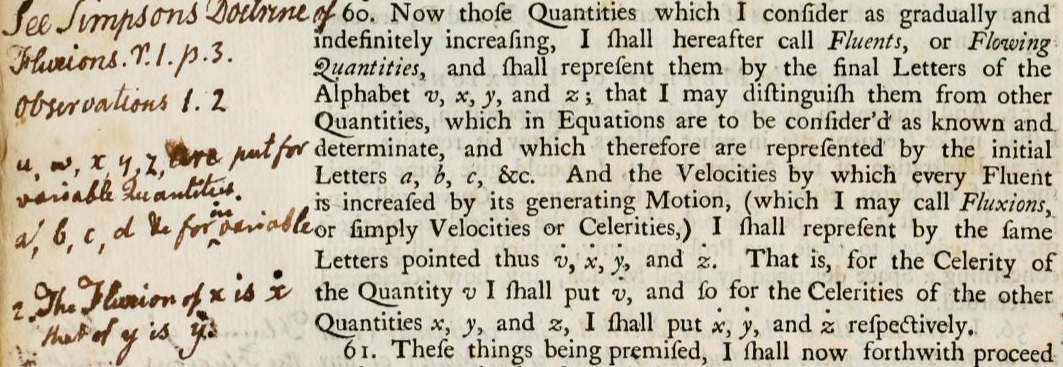
Figure 1. Newton's definitions for fluents and fluxions in The Method of Fluxions and Infinite Series [New2, p. 20] (pub. 1736), with John Adams’s handwritten notes in the margin. This particular volume is in the John Adams Library at the Boston Public Library. Image courtesy of Archive.org.

In Figure 1, we see a fully-formed theory of fluents and fluxions, Newton’s way of describing variable quantities and their instantaneous rates of change. Interestingly, this image [New2, p. 20] includes margin notes by John Adams, who apparently read this text in combination with Thomas Simpson’s 1737 book, Doctrine and Application of Fluxions [Sim], some pages of which feature as a Convergence Mathematical Treasure. Following Adams’s cryptic margin note, we find an equivalent definition of fluxions from Simpson on page 3 of Part I of the Doctrine and Application of Fluxions. By this time, Newton’s notation predominated in Britain, and Simpson’s work is no exception. Simpson’s first example of the utility of Newton’s notation is the calculation of the fluxion of x².

Figure 2. In his Doctrine and Application of Fluxions [Sim, p. 3], (pub. 1737), Thomas Simpson used a typical combination of geometric and analytic exposition to find the fluxion for x². Image courtesy of HathiTrust Digital Library.

Significantly, we see here how geometric the mathematical sciences still were; this preference for geometric arguments as the true justification for mathematical truths would continue well into the 19th century. So, too, would Newton's fluxional notation—English mathematician John Wallis adopted the notation in his 1693 text, De algebra tractatus [Wal], and extended it to include higher-order derivatives.

Figure 3. John Wallis's extension of Newton's ‘overdot’ notation to higher-order fluxions, from De algebra tractatus [Wal, p. 392] (pub. 1693). Image courtesy of HathiTrust Digital Library.

Here we see a proliferation of dots, denoting second-order, third-order, and even fourth-order derivatives! It should be noted that Newton himself used this extended notation in Tractatus de quadratura curvarum (pub. 1704), which he wrote in the same year that Wallis’s De algebra tractatus was printed.

At the same time that these geometers were developing the fluxional calculus in Britain, Leibniz and his disciples were exploring the same notational questions for their differential calculus. Returning to Cajori [Caj, p. 204], we find that Leibniz used a lower-case d for the differential as early as 1675, though it did not appear in print until 1684. That year, his “Nova methodus pro maximis et minimis” (“New method for finding maxima and minima”) was published in the Acta Eruditorum [Lei]. In it, Leibniz presented a method of calculating the tangents to a curve, including rules that would be familiar to any student of Calculus today: differentiating constant multiples, sums and differences, products, quotients and powers. Of course, Leibniz did not employ the now-common analytic geometry of functions and coordinates, instead using a geometric approach reminiscent of René Descartes’ La Géometrie. For a given point on a curve, Leibniz determined the length of a tangent line segment from the ratio of the point's “ordinate” to its “abscissa.” (In more modern language, we would say that Leibniz’s abscissa is a distance measured along the vertical coordinate axis, and the ordinate is the length of the perpendicular connecting the curve to the vertical coordinate axis.)

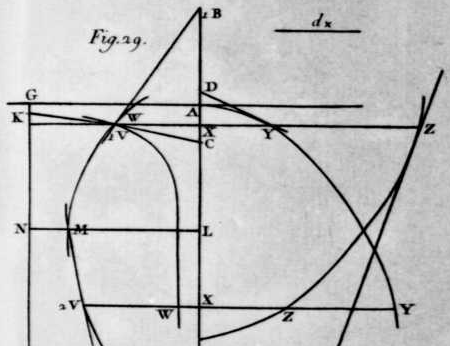
Figure 4. The geometric problem from Leibniz’s “Nova methodus pro maximis et minimis” [Lei] (pub. 1684), as it was reprinted in his collected works. Image courtesy of HathiTrust Digital Library.

While Leibniz used four curves to explain his method, we focus on one—the curve YYA in Figure 4. For this early version of the characteristic triangle, Leibniz constructed the line YD tangent to YYA, taking the ratio dy:dx = YX:YD to define the differential of y (the process was similar for the other variables v, w, z). Thereafter, he used an overline (also known as a vinculum) to denote the quantity whose differential he wished to find. Here is how some typical differentiation rules appeared in this notation:

• the constant multiple rule \(d\overline{ax} = a dx\),

• an addition and subtraction rule \(d\overline{z-y+w+x} = dz-dy+dw+dx\),

• the multiplication rule \(d\overline{xv} = x\,dv+v\,dx\).

In fact, Leibniz went as far as calculating second-order differentials—in his words, the “differences of the differences”—using the double-d notation (e.g., ddv). This notation is limited by Leibniz’s conception of the geometric quantities involved, but his new method for tangents was given a clear and consistent notation from the beginning.

Differences of Differences

As the decades passed, Newton’s fluxional Calculus held sway in Britain, while Leibniz’s differential predominated in continental Europe. One of the most prominent inheritors of the differential was Johann Bernoulli, the Swiss-born brother of Jakob and the mind behind the Marquis de L'Hôpital’s Analyse Infinitments Petits (pub. 1696), the first printed Calculus textbook. Here, we look at an excerpt from his 1694 article, "Effectionis omnium quadraturarum & rectificationum curvarum per seriem quandam generalissimam" [Ber1]. Following Leibniz’s use of d for differences and dd for “differences of the differences,” Bernoulli used the notations ddd and dddd in his derivation of a power series for \(x = b^{y/a}-a\).

Figure 5. Johann Bernoulli used multiple d’s to denote higher-order differentials in the power series for \(x = b^{y/a}-a\), in the 1694 paper, “Effectionis omnium quadraturarum & rectificationum curvarum per seriem quandam generalissimam” [Ber1, pp. 126-127]. Image courtesy of Google Books.

Parsing Bernoulli’s analysis, we see that he began with the ratio \(dy = a dx : r\), equivalent to \(\frac{dy}{dx} = \frac{a}{r}\), and used successive differentiation to obtain a series representation for y. In fact, Bernoulli did more than this—he used r = a+x, and while he did not evaluate the integral of dy, we know that \(y=a\cdot \ln(a+x)\) is an antiderivative. So in today's terminology, Bernoulli’s series representation is a Taylor series representation of a logarithm function. Taking a wider view, we can see here how the differential has now grown to include purely analytic methods, without direct consideration of curves and tangents.

At roughly the same time Bernoulli was writing the "Effectionis," he and Leibniz were corresponding with each other on the Calculus, and it is here that we get some clarity on their notational methods. In 1698, Leibniz wrote to Bernoulli suggesting that, when z is a function of x, the ratio of differences dz/dx be denoted with a ‘broken d’ notation—a dz with a horizontal line struck through the d, as we see below [Per, p. 526].

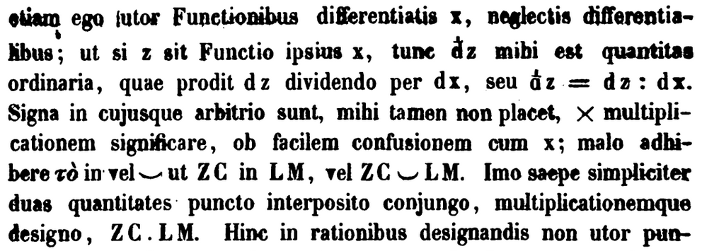
Figure 6. In a 1698 letter to Johann Bernoulli, Leibniz described his use of a ‘broken d’ notation for the difference ratio dz/dx. Image courtesy of HathiTrust Digital Library.

Perhaps the horizontal line was meant to evoke a fraction. At any rate, Bernoulli responded enthusiastically [Per, p. 531]:

Figure 7. Bernoulli’s response to Leibniz’s ‘broken d’ notation for denoting a ratio of differences (1698), indicating that he had used D for this purpose. Image courtesy of HathiTrust Digital Library.

Even though Bernoulli expressed his preference for Leibniz’s notation, the broken dz has not persisted. According to Cajori [Caj, p. 182], Leibniz never used the broken d in his published work, providing “a fine example of masterful self-control.” As we will see, it is Bernoulli’s capital D that persists in many of today's Calculus textbooks.

Delta, Del, and Nabla

As any student of multivariable Calculus knows, the letter d is not the end of this story. Today, the symbols \(\Delta\) and \(\nabla\) are often used to describe the theory of differentials in a higher-dimensional setting. Additionally, the Greek \(\Delta\) (capital delta) is known to students of pre-Calculus and physics as another way to represent change in a quantity. My own experience with \(\Delta\) as a student was that it denoted discrete (that is, not infinitesimal) differences: so \(\Delta y/\Delta x\) would represent the change in \(y\) with respect to \(x\) over a fixed interval, while \(dy/dx\) would represent the change in \(y\) with respect to \(x\) at an instant. However, the earliest uses of \(\Delta\) were less precise. For example, Johann Bernoulli published a solution to an isoperimetric problem in 1706 (originally posed by Bernoulli himself in 1697) in which he made use of \(\Delta\) to describe a continuous change.

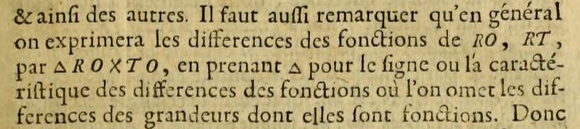
Figure 8. Johann Bernoulli's use of \(\Delta\) in his solution to an isoperimetric problem, published in the Paris Mémoires for 1706 [Ber2]. Image courtesy of Biodiversity Heritage Library.

Roughly translated, Bernoulli used \(\Delta\) to denote the “symbol for the differences of the functions where one omits the differences of the magnitudes of which they are functions.” Nearly 200 years later, the Swedish mathematician and historian Gustaf Eneström [Ene, p. 21] explained Bernoulli’s cumbersome language in this way:

\(\Delta RO\) is not the difference of RO, but the difference of a certain function of RO; moreover, we find easily that here, the word "difference" does not refer to a finite difference, but corresponds to the modern term "derivative," and consequently, the symbol \(\Delta\) must be defined not by the equation \(\Delta f(x) = f(x+h)-f(x)\), where \(f(x)\) is an arbitrary function, but by the equation \(\Delta x = \frac{df(x)}{dx}\), where \(f(x)\) is a function known in advance.

So, at this early stage, \(\Delta\) was a generalized differential that applied to a function of x. Also, the perceptive reader might notice the appearance of the word function in Bernoulli’s paper. While the notation for it came later, we see here an intuitive use of the word for any quantity that is dependent on another.

Through the 18th century, writers from Leonhard Euler to Maria Agnesi to Joseph-Louis Lagrange employed versions of the lower-case d for differentials in their work on Calculus. However, the usage of this notation had changed considerably from Leibniz’s day. One of the more underrated notational changes came from Alexis Fontaine, who wrote a manuscript in 1738 in which he introduced the familiar “fraction form” for ratios of differences, which allowed for the writer to express partial derivatives more clearly. While this manuscript was not published until 1764, knowledge of Fontaine’s contributions circulated widely during this time, eventually being adopted by most mathematicians of the day. One early mention of the fraction notation was in a 1740 letter by Alexis Clairaut to Euler [OO, pp. 68-69]:

Mr. Fontaine states the general method: \(\mu\) being an arbitrary function of \(x\) and \(y\), the difference of \(\int\mu\,dx\) in varying \(y\) and keeping \(x\) constant is \(dy \int\frac{d\mu}{dy} dx\); we mean by \(\frac{d\mu}{dy}\) the quantity which we obtain from differentiating \(\mu\), with variable \(y\) and \(x\) remaining constant...

Clairaut went on to explain how this notation unlocked the possibility of representing partial derivatives for functions of several variables. When Fontaine’s manuscript was printed 24 years later in the Paris Mémoires, we can see he made this exact point in “Le Calcul Intégral.”

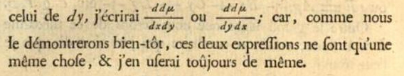
Figure 9. Fontaine's notation for differentials in "Le Calcul Intégral," a widely-read manuscript written in 1738 and only printed in 1764. Image courtesy of Google Books.

Identifying \(\mu\) as a function of variables \(p\), \(x\), \(y\), \(z\), etc., Fontaine described \(\frac{d\mu}{dx}\) as “the coefficient of \(dx\) in the differential of \(\mu\),” which is essentially the same as a partial derivative. We can see here that he went on to apply his notation to higher-order partial derivatives, even going as far to note the equality of the mixed partials \(\frac{dd\mu}{dx dy}\) and \(\frac{dd\mu}{dy dx}\).

A modern reader will notice the absence of the symbol \(\partial\) in Fontaine's notation. Indeed, this symbol seems to find its origin in a 1786 paper by Adrien-Marie Legendre [Leg]. In his “Mémoire sur la manière de distinguer les maxima des minima dans le Calcul des Variations” (“Memoir on the method for distinguishing maxima and minima in the Calculus of Variations”), Legendre used the Greek \(\delta\) to represent the total differential, with the variant \(\partial\) representing partial derivatives in the calculation.

Figure 10. In the 1786 paper, “Mémoire sur la manière de distinguer les maxima des minima dans le Calcul des Variations” [Leg], Legendre modified Fontaine's notation, using \(\partial\) and \(\delta\) for partial differentials. Image courtesy of the Bibliothèque Nationale de France's Gallica collection.

In a footnote marked with a (*) in the image above, Legendre explained his use of this symbol:

To avoid any ambiguity, I will represent by \(\frac{\partial v}{\partial x}\) the coefficient of dx in the differential of v, and by \(\frac{dv}{dx}\) the complete differential of v divided by dx.

So we see that, by the close of the 18th century, the notation for differentials had expanded to include multivariate functions, with notions of total and partial differentials having their own symbols. What began with Leibniz's simple dx in the "Nova methodus pro maximis et minimis" now included D, \(\Delta\), \(\partial\), \(\delta\), each with their varying contexts.

Diverging Derivatives

As Calculus advanced into the 19th century, many new developments expanded the notion of “change” in the minds of mathematicians. In particular, this included the incorporation of the vector concept into Calculus, providing many new ways of defining differentials for more sophisticated situations. To close out this article (and this series), we take a brief tour of the various differential notations that have appeared in multivariate Calculus in the past two centuries.

We have already seen that, as early as 1706, Johann Bernoulli used the Greek letter \(\Delta\) to denote the derivative for a single-variable function. However, many students of vector Calculus know this symbol as the cousin of \(\nabla\)—variously called del or nabla—used to denote the divergence of a vector field. Specifically, for a vector field \(\vec{F} = \langle F_x, F_y, F_z\rangle\), the divergence may be denoted by \(\nabla\cdot\vec{F}\), which is to say that the operator \(\nabla=\langle\frac{\partial}{\partial x}, \frac{\partial}{\partial y}, \frac{\partial}{\partial z}\rangle\) is combined with \(\vec{F}\) using a formal inner product. Informally, the divergence measures the extent to which the vector field “pushes” out of a given region. Since our interest lies in the symbols used to represent this concept, it is worth noting that the inverted \(\Delta\) was not the only way this concept has been expressed. William Rowan Hamilton used a sideways \(\Delta\) in his paper, “On the Expression and Proof of Paschal’s Theorem by Means of Quaternions” [Ham] which appeared in the Royal Irish Academy's Proceedings for the years 1845–1847. Here is Hamilton's original definition from page 291, written from the perspective of the Academy:

the following more general characteristic of operation,

\(i\frac{\text{d}}{\text{d}x}+j\frac{\text{d}}{\text{d}x}+k\frac{\text{d}}{\text{d}x} = {\Large \triangleleft}\),

in which \(x\), \(y\), \(z\) are the ordinary rectangular coordinates, while \(i\), \(j\), \(k\) are his own coordinate imaginary units, appears to him to be one of great importance in many researches. This will be felt (he thinks) as soon as it is perceived that with this meaning of \({\Large \triangleleft}\) the equation

\(\left(\frac{\text{d}}{\text{d}x}\right)^2+\left(\frac{\text{d}}{\text{d}y}\right)^2+\left(\frac{\text{d}}{\text{d}z}\right)^2 = -{\Large \triangleleft}^2\),

is satisfied in virtue of the fundamental relations between his symbols \(i\), \(j\), \(k\).

A version of Hamilton's notation was adopted by Peter Tait in his 1867 text, An Elementary Treatise on Quaternions, though by that time the \(\Delta\) symbol had completed its rotation to become \(\nabla\). Beginning on p. 221, Tait carried out a nearly-identical calculation to that of Hamilton, applying the operator \(\nabla\) to a vector field for the first time:

Figure 11. Peter Tait inverted \(\Delta\) to use \(\nabla\) in An Elementary Treatise on Quaternions [Tai, p. 221] (pub. 1867). Image courtesy of Archive.org.

We see the \(\nabla\) symbol is first used to denote Hamilton’s differential operator, and then repeated to produce the now-named Laplace operator \(\nabla^2\). As to the symbol itself, it is sometimes named as “del” or “nabla,” with the former being an abbreviation of the word “delta.” The latter was suggested to Tait by the biblical scholar and encyclopedist William Robertson Smith, who was inspired by the Greek \(\nu\alpha\beta\lambda\alpha\), meaning “harp,” since he considered the inverted \(\Delta\) to resemble a harp.

As with all good origin stories, the picture becomes blurred as time passes. By the late 19th century, many different symbols were in use across the world, and while some early symbol choices (like Leibniz’s “broken d”) were rejected, many others had their acolytes. Many in Britain, including many physicists, continued to use Newton’s overdot notation—and many still do! Others use Leibniz’s d for single-variable Calculus, but adopt \(\partial\) and \(\nabla\) when in a multivariable setting. And while the capital letter \(\Delta\) is often reserved for discrete differences, this rule is not always strictly observed.

As to the capital D, it achieved a minor renaissance in the United States due to a historical accident. Before the 19th century, the Calculus done in the British colonies was heavily Newtonian (as suggested by Adams’ reliance on Newton’s fluxions in his studies). This began to change in the early 19th century. In particular, the American mathematician Benjamin Peirce adopted the capital D as his primary notation for the derivative in his 1841 text, Curves, Functions, and Forces. Peirce, a long-serving Harvard professor and an influential mathematical figure in the early years of the United States, saw his notation adopted at schools across the country. While the capital D no longer retains the central role in American classrooms that it once did, it does show that sometimes a notational choice is more of an accident than a true choice.

References

[Ber1] Bernoulli, Johann. "Effectionis omnium quadraturarum & rectificationum curvarum per seriem quandam generalissimam." Johannis Bernoulli Opera Omnia, Vol. 1, pp. 125–128. Lausanne and Geneva, 1742.

[Ber2] Bernoulli, Johann. "Du Problême proposé par M. Jacques Bernoulli dans les Actes de Leipsik du mois de May de l'année 1697." Mémoires de à l'Académie Royale des Sciences, année 1706 (1731), 235–245.

[Caj] Cajori, Florian. A History of Mathematical Notations. Vol. 2. Chicago: Open Court Publishing Co., 1928.

[Ene] Eneström, Gustaf. "Recensionen – Analyses." Bibliotheca Mathematica, Series 2, 10 (1896), 17–26.

[Fon] Fontaine, Alexis. "Le Calcul Intégral." Mémoires donnés à l'Académie Royale des Sciences, non imprimés dans leur temps (1764), 24–28.

[Gra] Grabiner, Judith. "The Changing Concept of Change: The Derivative from Fermat to Weierstrass." Math. Magazine 56 (no. 4) (1983), 295–206.

[Ham] Hamilton, William Rowan. "On the Expression and Proof of Paschal's Theorem by Means of Quaternions." Proceedings of the Royal Irish Academy (1836–1869) 3 (1844–1847), 273–294.

[Hun] Hunachek, Mark. Review of The History of the Priority Dispute between Newton and Leibniz, by Thomas Sonar. MAA Reviews, 12 June 2018.

[Leg] Legendre, Adrien-Marie. "Mémoire sur la manière de distinguer les maxima des minima dans le Calcul des Variations." Mémoires de à l'Académie Royale des Sciences (1786), 7–37.

[Lei] Leibniz, Gottfried. "Nova Methodus Pro Maximis et Minimis, itemque tangentibus, que nec fractas, nec irrationales quantitates moratur, et singulare pro illis calculi genus." Acta Eruditorum (1684), 467–473.

[New1] Newton, Isaac. De Analysi per aequationes numero terminorum infinitas. Letter to John Collins, 31 July 1669. Published in London: William Pearson, 1711.

[New2] Newton, Isaac. The Method of Fluxions and Infinite Series. London: Henry Woodfall, 1736.

[OO] Lemmermeyer, F. and M. Mattmuller, eds. Leonhard Euler Opera Omnia: Series Quarta A. Volume 5: Commercium Epistolicum. Basel: Springer, 1980.

[Per] Pertz, Georg H., ed. Leibnizens gesammelte Werke. Vol. 3. Halle: H. W. Schmidt, 1856.

[Sim] Simpson, Thomas. The Doctrine and Application of Fluxions. London: Knight and Compton, 1737.

[Son] Sonar, Thomas. The History of the Priority Dispute between Newton and Leibniz. Birkhäuser, 2018.

[Tai] Tait, Peter. An Elementary Treatise on Quaternions. Oxford: Clarendon Press, 1867.

[Wal] Wallis, John. De algebra tractatus. Oxford, 1693.