Geometric Photo Manipulation
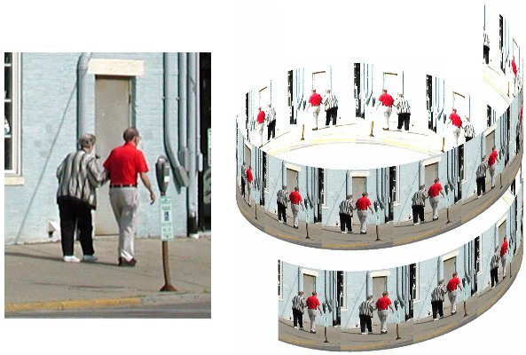
Figure 1
Tom Farmer is Associate Professor of Mathematics at Miami University.
I present here a way that students of calculus and linear algebra can use both artistic and mathematical abilities to transform ordinary photographs into interesting pictures having mathematical content. As a quick illustration, Figure 1 shows copies of an input photo tracing the path of a helix and viewed as if they were pasted onto an invisible cylinder. Similarly, almost any three dimensional object that you can imagine -- if you can describe it by mathematical formulas -- might be "colored" using a given photo. This idea is timely, not only because computer graphics is a rapid growth area that is notable for its uses of mathematics, but also because we now have easy access to digital photographic images via digital cameras and scanners.
Published October, 2002
© 2002, Thomas A. Farmer
Geometric Photo Manipulation - Introduction
Figure 1
Tom Farmer is Associate Professor of Mathematics at Miami University.
I present here a way that students of calculus and linear algebra can use both artistic and mathematical abilities to transform ordinary photographs into interesting pictures having mathematical content. As a quick illustration, Figure 1 shows copies of an input photo tracing the path of a helix and viewed as if they were pasted onto an invisible cylinder. Similarly, almost any three dimensional object that you can imagine -- if you can describe it by mathematical formulas -- might be "colored" using a given photo. This idea is timely, not only because computer graphics is a rapid growth area that is notable for its uses of mathematics, but also because we now have easy access to digital photographic images via digital cameras and scanners.
Published October, 2002
© 2002, Thomas A. Farmer
Geometric Photo Manipulation - Images as Data
The geometric manipulations we have in mind are applied to data in the form of photographic images, and we carry out the manipulations using MATLAB or perhaps another programming language. We require that the software can open an image file as an array of numbers that can be manipulated. This initial step is complicated by the fact that there are several "modes" of images and several common file types. In order to get quickly to my main focus, I will assume that the reader has an image in RGB mode that is saved as a JPEG file. (RGB means "red, green, and blue" and indicates that the image is a standard color image. JPEG stands for Joint Photographic Experts Group and is a standard image compression routine.) Most images that come from the internet or from a digital camera are apt to be in that form already. And, if not, then many graphics applications that you might use to crop a photo or to adjust the brightness and contrast also allow you to put the image into RGB mode and to save it as a JPEG file.
An RGB image can be thought of as a rectangular array of "elements", one for each pixel of the image, where each element is a triple of numbers representing the red, green, and blue intensities of the pixel. The numbers used in each triple are typically required to be in the interval ![]() , with
, with ![]() representing black and
representing black and ![]() white. However, just to complicate matters a little more, it seems to be a common convention that the numbers are stored as 8-bit integers from 0 to 255. These integers are ultimately divided by 255 to yield values in
white. However, just to complicate matters a little more, it seems to be a common convention that the numbers are stored as 8-bit integers from 0 to 255. These integers are ultimately divided by 255 to yield values in ![]() .
.
The JPEG compression routine has little impact in this discussion -- once the image is read into the computer's memory as an array, the array size is the same whether or not there had been any compression in the stored file. Thus, a shot from a 3 megapixel digital camera may yield a 1536 by 2048 array, which is saved as a compressed JPEG file of only 1 megabyte. But when the file is opened in MATLAB it becomes, once again, an array of the original size. By the way, a supercomputer may be needed to work with image files of that size in MATLAB -- let's experiment first with arrays that are just a few hundred pixels on a side.
Geometric Photo Manipulation - Projections
Analytic geometry of the sort usually found in multivariable calculus enters our discussion as we imagine displaying a three dimensional object on a two-dimensional computer screen or photographic print. Figure 2 depicts the two most common ways of accomplishing such a projection.
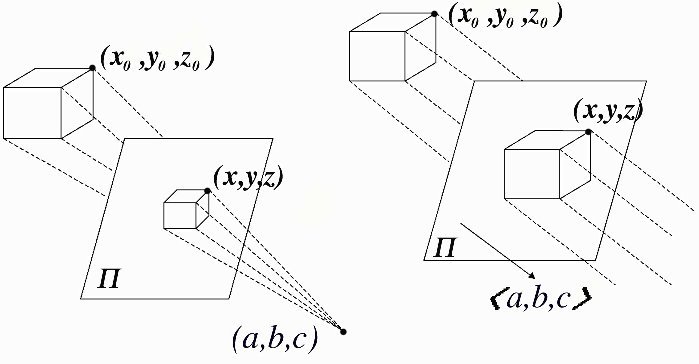
(a) Perspective projection (b) Orthographic projection
Figure 2
- In perspective projection [Figure 2(a)], we imagine that the eye of an observer is at a point
 that is neither a point of the object (the cube) nor a point of a given plane
  , where the scene will be projected. Then any point
  of the object is projected to the point where the line through
  and
and  meets the plane
  . The final step is to coordinatize this plane so as to identify its points with the pixels of the output image.
- In orthographic projection [Figure 2(b)], we imagine that the eye of the observer is at infinity, and the observer views the scene along a fixed direction vector
 . This time, each point
  of the scene is projected to the point where the line through
  with direction vector
  meets a given plane
  (a plane with normal vector
  ).
).
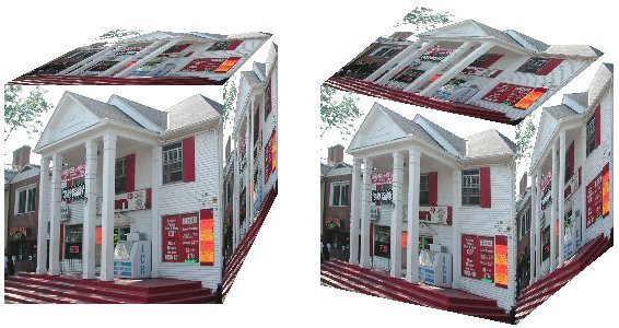
(a) Perspective projection (b) Orthographic projection
Figure 3
As one can see from Figure 3, a cube drawn with a perspective projection has back edges that are smaller in size than the front edges, suggestive of the greater distance from the eye. In contrast, the orthographic projection yields front and back edges of the same size. Both projection methods are fundamental in computer graphics, and I think a discussion of them can provide a compelling application of certain topics from calculus and linear algebra.
Geometric Photo Manipulation - Projection Formulas: Perspective
To clarify the projection methods, let's look in more detail at the example shown in Figure 3 (preceding page), in which the 400 by 400 pixel image of a storefront is pasted onto three faces of a cube in ![]() . The cube is our three-dimensional object -- its front face is the plane
. The cube is our three-dimensional object -- its front face is the plane ![]() , and the other faces are the planes
, and the other faces are the planes ![]() and
and ![]() . To project this object -- using either the perspective or the orthographic method -- we apply the color values of the
. To project this object -- using either the perspective or the orthographic method -- we apply the color values of the ![]() pixel (counting i rows down from the top and j columns left to right in the input image) to each of three points belonging to the three visible faces of the cube. That is, letting
pixel (counting i rows down from the top and j columns left to right in the input image) to each of three points belonging to the three visible faces of the cube. That is, letting ![]() be
be ![]() for the front face,
for the front face, ![]() for the right face, and
for the right face, and ![]() for the top face, we apply the color of the
for the top face, we apply the color of the ![]() pixel to a certain computed point of the output image.
pixel to a certain computed point of the output image.
For the perspective projection in Figure 3(a), the viewer's eye is at the point ![]() , and the viewing plane is
, and the viewing plane is ![]() . In this case, we find that the computed point
. In this case, we find that the computed point ![]() where the line through
where the line through ![]() and
and ![]() meets the viewing plane is
meets the viewing plane is
In the final step we need to identify these projected points with the pixels of an output image. One way is to begin by (roughly) estimating bounds on the calculated y and z coordinates. Let's say that all the points ![]() calculated from the scene satisfy
calculated from the scene satisfy ![]() and
and ![]() . Then we can use
. Then we can use ![]() to yield appropriate row and column indices for the output image. Note that the indices are chosen so that the largest possible z value in the scene leads to the smallest row number (at the top of the image) and the smallest y value of the scene leads to the smallest column number (at the left edge of the image). The function round is applied to round to the nearest integer so that the indices of the output array are positive integers. The size of the output array can be taken to be
to yield appropriate row and column indices for the output image. Note that the indices are chosen so that the largest possible z value in the scene leads to the smallest row number (at the top of the image) and the smallest y value of the scene leads to the smallest column number (at the left edge of the image). The function round is applied to round to the nearest integer so that the indices of the output array are positive integers. The size of the output array can be taken to be ![]() rows and
rows and ![]() columns.
columns.
This procedure has been implemented in the MATLAB program perspective.m.
Geometric Photo Manipulation - Projection Formulas: Orthographic
To derive the formula for the orthographic projection method, we need some linear algebra. In our example, Figure 3(b), the line of sight from the scene to the eye at infinity has direction vector ![]() . For convenience, we let
. For convenience, we let ![]() be the spherical coordinates of the point
be the spherical coordinates of the point ![]() , and we let
, and we let ![]() . As we might expect, the formula for the projection turns out to depend only on the angles
. As we might expect, the formula for the projection turns out to depend only on the angles ![]() and
and ![]() and not on the magnitude of
and not on the magnitude of ![]() .
.
Orthographic projection, unlike perspective projection, can be treated as a linear transformation -- it's the orthogonal projection T from ![]() to
to ![]() whose image is the plane
whose image is the plane ![]() given by
given by ![]() . Perhaps the clearest way to derive the formula for the projection is to find an orthonormal basis
. Perhaps the clearest way to derive the formula for the projection is to find an orthonormal basis ![]() for
for ![]() such that the first two vectors span the plane
such that the first two vectors span the plane ![]() . To begin, let
. To begin, let ![]() denote the usual basis for
denote the usual basis for ![]() , and define
, and define
which is a unit vector normal to the plane ![]() . Next (assuming
. Next (assuming ![]() is not parallel to
is not parallel to ![]() ), we take
), we take
![]() .
.
This is a unit vector orthogonal to ![]() , therefore is in the subspace
, therefore is in the subspace ![]() . Finally, letting
. Finally, letting
![]() ,
,
we get an orthonormal basis ![]() for
for ![]() . Now for any vector v, the orthogonal projection is given by
. Now for any vector v, the orthogonal projection is given by ![]() , because this map sends
, because this map sends ![]() to zero and leaves fixed any vector in the subspace
to zero and leaves fixed any vector in the subspace ![]() . In terms of
. In terms of  , we have
and the coefficients C1 and C2 coordinatize ![]() .
.
The final step is to connect this result with the pixels of the output image. Just as we did with the perspective method, we estimate bounds for the calculated components of ![]() corresponding to points of the three-dimensional object -- let's say
corresponding to points of the three-dimensional object -- let's say ![]() and
and ![]() for all points
for all points ![]() of the object. Then
of the object. Then ![]() and
and ![]() yield appropriate row and column indices for an output image, and the size of the image can be taken to be
yield appropriate row and column indices for an output image, and the size of the image can be taken to be ![]() rows and
rows and ![]() columns.
columns.
This procedure has been implemented in the MATLAB program orthographic.m.
Geometric Photo Manipulation - Hidden Points: The z-buffer
The particular examples of Figure 3 avoid the problem of having parts of the object that should be hidden from view (unless the line-of-sight is chosen carelessly). If we had painted all six faces of the cube, though, there would often be two distinct points ![]() and
and ![]() of the object that are projected to the same point in the viewing plane. But only the point that is nearest to the viewer's eye should be visible. Fortunately, this problem has a well-known solution in computer graphics called a z-buffer, an array having the same row and column dimensions as the output array. For each pixel of the output image, the buffer stores a value representing the distance from a point of the three-dimensional object to the viewer's eye (or to an appropriate plane if the eye is at infinity). The z-buffer can be initialized with values that are larger than any distance that arises from the object. Then the color of an output pixel is changed only if the distance from the given point
of the object that are projected to the same point in the viewing plane. But only the point that is nearest to the viewer's eye should be visible. Fortunately, this problem has a well-known solution in computer graphics called a z-buffer, an array having the same row and column dimensions as the output array. For each pixel of the output image, the buffer stores a value representing the distance from a point of the three-dimensional object to the viewer's eye (or to an appropriate plane if the eye is at infinity). The z-buffer can be initialized with values that are larger than any distance that arises from the object. Then the color of an output pixel is changed only if the distance from the given point ![]() to the eye is smaller than the value held in the z-buffer. If this is the case, the value in the buffer is updated to be the distance just computed. This device is further described in the next section, and code to implement it is included in the programs perspective.m and orthographic.m.
to the eye is smaller than the value held in the z-buffer. If this is the case, the value in the buffer is updated to be the distance just computed. This device is further described in the next section, and code to implement it is included in the programs perspective.m and orthographic.m.
Geometric Photo Manipulation - The Algorithm Explained
The MATLAB programs perspective.m and orthographic.m are designed to produce the cube pictures of Figure 3, but the programs can be altered to generate an unlimited number of constructions, for example, the one in Figure 1 and those to appear in the next section. Here is an outline for such programs:
-
The beginning:
- Read the input image data into memory as an array. Let's call it inpic.
- Assign values to the parameters required by the perspective projection method. (We limit this outline to the perspective case, but the orthographic method has a very similar outline.) It's a good idea to express these values in terms of the dimensions of the input image so that one can experiment first with a very small input image and easily switch later to a larger image. This is important because programs can take a long time to run if the input image is large.
- Assign values to the estimated bounds on the calculated projection points, and initialize the output array called outpic by assigning the value "white" to each pixel. Also initialize the values of the z-buffer array.
-
The middle:
- Loop just once through the pixels of the input image. For each pixel
 , enter formulas for the desired positions
  of the envisioned object
-- there will be one set of formulas for each copy of the image that is to be included in the object (e.g., the three visible faces of the cube in Figure 3). This is the primary way in which one construction differs from another. For each point , do the following:
- Calculate the projected point and the corresponding output array address;
- Compute the distance from
 to the point
  , and proceed to (c) only if the distance is smaller than the one held in the z-buffer for that output array address;
- Change the corresponding output array value (all three RGB levels) to inpic(i,j), and update the z-buffer value by assigning as the new value the distance computed in step b.
- The ending:
- Save and/or print the output array as an image.
Geometric Photo Manipulation - Examples
Generating pictures such as the ones in this article may require a little mathematics as well as a considerable amount of experimentation. For example, Figure 1 involves, among other things, expressing an arc of a helix in parametric form with arc length as the parameter. Parameterizations using some other parameter would be apt to deform the pictures or leave gaps. Figure 4 below requires that same type of parameterization for the circles that generate a torus; it is also an application of the tangent, normal, and binormal vectors of a parametric curve.
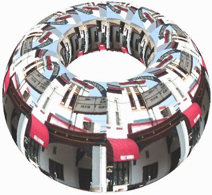
Figure 4
A picture like the one in Figure 5 can be a fun way to clarify a three-dimensional object. In this case we are able to visualize the shape of the solid obtained as the intersection of two cylinders arising from two input images.
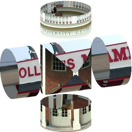
Figure 5
There is no end to the possible examples, and many are apt to lead to challenges that can pique students' interest in mathematical topics.
Geometric Photo Manipulation - Projects
- The Cube
- Copy and paste one of the programs perspective.m or orthographic.m into MATLAB, and apply it to one of your own picture files. Remember to reduce the size of the image to a few hundred pixels on a side, place the file in MATLAB's active directory, and enter the name of your file in the first line of the program.
- Alter the program of part (a) by deleting the section of commands pertaining to the "top face" of the cube and, instead, including sections for a "back face" in the plane
 and a "left face" in the plane
  . By running this altered program, you will see the effect of the z-buffer.
- Copy and paste one of the programs perspective.m or orthographic.m into MATLAB, and apply it to one of your own picture files. Remember to reduce the size of the image to a few hundred pixels on a side, place the file in MATLAB's active directory, and enter the name of your file in the first line of the program.
- The Cylinder
- Alter one of the programs perspective.m or orthographic.m to produce a right circular cylinder with vertical axis and with 3 copies of a picture wrapped side-by-side around it. A good start would be to parameterize the cylinder using two parameters, one representing arc length along the circular base and the other the height. If the dimensions of the input picture are row by col, then the cylinder should have height equal to row and circumference equal to 3*col. Thus, a section of the MATLAB code might be
for k=0:2
x0=((3*col)/(2*pi))*cos((2*pi*(k*col+j))/(3*col));
y0=((3*col)/(2*pi))*sin((2*pi*(k*col+j))/(3*col));
z0=row-i+1;
[perspective or orthographic procedure goes here]
end
The For Loop has k taking on values 0, 1, and 2 in order to produce the three copies of the image.
- Alter the program in part (a) to produce a horizontal cylinder with one copy of an input image showing on the front half and another copy on the back half. The front image should be upright.
- Alter one of the programs perspective.m or orthographic.m to produce a right circular cylinder with vertical axis and with 3 copies of a picture wrapped side-by-side around it. A good start would be to parameterize the cylinder using two parameters, one representing arc length along the circular base and the other the height. If the dimensions of the input picture are row by col, then the cylinder should have height equal to row and circumference equal to 3*col. Thus, a section of the MATLAB code might be
- The Helical Band
Alter one of the programs perspective.m or orthographic.m to produce a "helical band" similar to Figure 1. The pixels along the bottom row of
 copies of the input image are to be positioned along the helix initially parameterized by
  ,
,  , and
, and  , where r and m have to be suitably chosen. Start by re-parameterizing the helix by arc length. Then decide how many revolutions you want there to be (say
  ), and figure out what values of r and m will yield, in that many revolutions, an arc length equal to n times the number of columns of the input image. It may help to assume
  , but this ratio determining the slope of the helix can be adjusted. For simplicity, each column of pixels is to be sent to a vertical line segment starting at a point of the helix. It is a good idea to use variables such as n, r, m, and rev in the program so their values can easily be altered. Also, rather than having 19 separate sections of code in the program for the 19 copies of the input image, it works well to use a For Loop letting an index k take values from 0 to n-1.
 -
The Torus
Alter one of the programs perspective.m or orthographic.m to produce a torus as in Figure 4. Twenty copies of an input image that is about 50% taller than it is wide are used in that figure, but you should feel free to experiment with other choices. Let's think of a torus as a surface obtained by rotating about the z-axis a circle of radius r whose center C is in the xy-plane R units from the z-axis (with
 ). Let's assume that the dimensions of the input image are row by col, and we intend to wrap the torus with what amounts to a 2 by 10 array of copies of the image. Then it may work well to require
  and
and  . Note that as the center C is rotated about the z-axis, it produces a circle of radius R that can be parameterized by
  ,
,  , and
, and  . Also, t can be assigned
  equally spaced values from 0 to 2
 , and, for each value of t, the point
  is the center of a circle of radius r along which we want to position a column of pixels. The unit normal and binormal vectors of the parameterized R-circle offer a handy way to find the coordinates of the points on these r-circles.