This module is designed for use in a first-semester differential calculus course to stimulate interest in the derivative as a tool for modeling rate of change.

Notes for the Instructor

About this Module and its Authors

Choice of Computer Algebra System

Click on the button corresponding to your preferred computer algebra system (CAS). This will download a file which you may open with your CAS.
 

Ver. 6 or higher

Ver. 3.0 or higher

Ver. 5.1 or higher

 

Copyright 2000, CCP and the authors

Published December, 2001

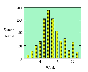
During the winter of 1968-1969, the United States was swept by a virulent new strain of influenza, named Hong Kong flu for its place of discovery. At that time, no flu vaccine was available, so many more people were infected than would be the case today. We will study the spread of the disease through a single urban population, that of New York City. The data displayed in the following table are weekly totals of "excess" pneumonia-influenza deaths, that is, the numbers of such deaths in excess of the average numbers to be expected from other sources. The graph displays the same data.  (Source: Centers for Disease Control. Click here for a recent CDC view of influenza pandemics.)

 

Week Flu-related deaths Week Flu-related deaths 1 14 8 108 2 28 9 68 3 50 10 77 4 66 11 33 5 156 12 65 6 190 13 24 7 156

  

Relatively few flu sufferers die from the disease or its complications, even without a vaccine. However, we may reasonably assume that the number of excess deaths in a week was proportional to the number of new cases of flu in some earlier week, say, three weeks earlier. Thus the figures in the table reflect (proportionally) the rise and subsequent decline in the number of new cases of Hong Kong flu. We will model the spread of such a disease so that we can predict what might happen with similar epidemics in the future.

At any given time during a flu epidemic, we want to know the number of people who are infected. We also want to know the number who have been infected and have recovered, because these people now have an immunity to the disease. (As a matter of convenience, we include in the recovered group the relative handful who do not recover but die -- they too can no longer contract the disease.) The remainder of the population is still susceptible to the disease. (We assume that the same people are in New York during the weeks of the epidemic -- that is, we ignore the relatively few who are born or die from non-flu causes or move into or out of the city during those weeks.)

Thus, at any time, the fixed total population (approximately 7,900,000 in the case of New York City in the late 1960's) may be divided into three distinct groups:

• those who are infected,
• those who have recovered, and
• those who are still susceptible.

In the next part, we will investigate a simple model that accounts for a few of the features of the spread of a disease such as the Hong Kong Flu.

As the first step in the modeling process, we identify the independent and dependent variables. The independent variable is time  t,  measured in days. We consider two related sets of dependent variables.

The first set of dependent variables counts people in each of the groups, each as a function of time:

S = S(t)	is the number of susceptible individuals,
I = I(t)	is the number of infected individuals, and
R = R(t)	is the number of recovered individuals.

The second set of dependent variables represents the fraction of the total population in each of the three categories. So, if  N  is the total population (7,900,000 in our example), we have

s(t) = S(t)/N,	the susceptible fraction of the population,
i(t) = I(t)/N,	the infected fraction of the population, and
r(t) = R(t)/N,	the recovered fraction of the population.

It may seem more natural to work with population counts, but some of our calculations will be simpler if we use the fractions instead. The two sets of dependent variables are proportional to each other, so either set will give us the same information about the progress of the epidemic.

1. Under the assumptions we have made, how do you think  s(t)  should vary with time? How should  r(t)  vary with time? How should  i(t)  vary with time?

2. Sketch on a piece of paper what you think the graph of each of these functions looks like.

3. Explain why, at each time  t,  s(t) + i(t) + r(t) = 1.

Next we make some assumptions about the rates of change of our dependent variables:

• No one is added to the susceptible group, since we are ignoring births and immigration. The only way an individual leaves the susceptible group is by becoming infected. We assume that the time-rate of change of  S(t),  the number of susceptibles,¹ depends on the number already susceptible, the number of individuals already infected, and the amount of contact between susceptibles and infecteds. In particular, suppose that each infected individual has a fixed number  b  of contacts per day that are sufficient to spread the disease. Not all these contacts are with susceptible individuals. If we assume a homogeneous mixing of the population, the fraction of these contacts that are with susceptibles is  s(t).  Thus, on average, each infected individual generates  b s(t)  new infected individuals per day. [With a large susceptible population and a relatively small infected population, we can ignore tricky counting situations such as a single susceptible encountering more than one infected in a given day.]

• We also assume that a fixed fraction  k  of the infected group will recover during any given day. For example, if the average duration of infection is three days, then, on average, one-third of the currently infected population recovers each day. (Strictly speaking, what we mean by "infected" is really "infectious," that is, capable of spreading the disease to a susceptible person. A "recovered" person can still feel miserable, and might even die later from pneumonia.)

Let's see what these assumptions tell us about derivatives of our dependent variables.

4. The Susceptible Equation. Explain carefully how each component of the differential equation
   
   

   (1)

   
   follows from the text preceding this step. In particular,
   
   
   • Why is the factor of  I(t)  present?

   • Where did the negative sign come from?
     
     
   Now explain how this equation leads to the following differential equation for  s(t).
   
   

   (2)

5. The Recovered Equation. Explain how the corresponding differential equation for  r(t),
   
   

   (3)

   
   follows from one of the assumptions preceding Step 4.

6. The Infected Equation. Explain why
   
   

   (4)

   
   What assumption about the model does this reflect? Now explain carefully how each component of the equation
   
   

   (5)

   
   follows from what you have done thus far. In particular,
   
   
   • Why are there two terms?

   • Why is it reasonable that the rate of flow from the infected population to the recovered population should depend only on  i(t)   ?

   • Where did the minus sign come from?

Finally, we complete our model by giving each differential equation an initial condition. For this particular virus -- Hong Kong flu in New York City in the late 1960's -- hardly anyone was immune at the beginning of the epidemic, so almost everyone was susceptible. We will assume that there was a trace level of infection in the population, say, 10 people.² Thus, our initial values for the population variables are

S(0) = 7,900,000

I(0) = 10

R(0) = 0

In terms of the scaled variables, these initial conditions are

s(0) = 1

i(0) = 1.27 x 10- 6

r(0) = 0

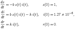
(Note: The sum of our starting populations is not exactly  N,  nor is the sum of our fractions exactly  1.  The trace level of infection is so small that this won't make any difference.) Our complete model is

(6)

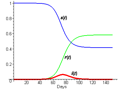
We don't know values for the parameters  b  and  k   yet, but we can estimate them, and then adjust them as necessary to fit the excess death data. We have already estimated the average period of infectiousness at three days, so that would suggest  k = 1/3.  If we guess that each infected would make a possibly infecting contact every two days, then  b  would be  1/2.  We emphasize that this is just a guess. The following plot shows the solution curves for these choices of  b  and  k. 

7. In steps 1 and 2, you recorded your ideas about what the solution functions should look like. How do those ideas compare with the figure above? In particular,
   
   
   • What do you think about the relatively low level of infection at the peak of the epidemic?

   • Can you see how a low peak level of infection can nevertheless lead to more than half the population getting sick? Explain.
     
     

In Part 3, we will see how solution curves can be computed even without formulas for the solution functions.

 

---

¹ Note that we have turned the adjective "susceptible" into a noun. It is common usage in epidemiology to refer to "susceptibles," "infecteds," and "recovereds" rather than always use longer phrases such as "population of susceptible people" or even "the susceptible group."

² While I(0) is normally small relative to N, we must have I(0) > 0 for an epidemic to develop. Equation (5) says, quite reasonably, that if I = 0 at time 0 (or any time), then dI/dt = 0 as well, and there can never be any increase from the 0 level of infection.

 

In Part 3, we displayed solutions of an SIR model without any hint of solution formulas. This suggests the use of a numerical solution method, such as Euler's Method, which we assume you have seen in the context of a single differential equation. Nevertheless, we review the basic idea here.

Recall the idea of Euler's Method: If we have a "slope formula," i.e., a way to calculate  dy/dt  at any point  (t,y),  then we can generate a sequence of y-values,

y₀, y₁, y₂, y₃, ...

by starting from a given  y₀  and computing each rise as slope x run. That is,

y_n = y_n-1 + slope_n-1 Delta_t

where  Delta_t  is a suitably small step size in the time domain.

It really doesn't matter in this calculation if the slope formula happens to depend not just on  t  and  y  but on other variables, say  x  and  z -- as long as we know how  x  and  z are related to  t  and  y.  If  x  and  z happen to be other dependent variables in a system of differential equations, we can generate values of  x  and  z in the same way.

Of course, for the SIR model, we want the dependent variable names to be  s,  i,  and  r.  Thus we have three Euler formulas of the form

s_n = s_n-1 + s-slope_n-1 Delta_t,

i_n = i_n-1 + i-slope_n-1 Delta_t,

r_n = R_n-1 + r-slope_n-1 Delta_t,

More specifically, given the SIR equations,

the Euler formulas become

Of course, to calculate something from these formulas, we must have explicit values for  b,  k,  s(0), 
i(0),  r(0),  and  Delta_t. In this part we explore the adequacy of these formulas for generating solutions of the SIR model. If your helper application has Euler's Method as an option, we will use that rather than construct the formulas from scratch.

1. In your helper application (CAS) worksheet, you will find commands to use the built-in differential equations solver. Use these commands, with the sample values of  b = 1/2  and  k = 1/3 in your worksheet, to generate graphical solutions of the SIR equations, starting from  s(0) = 1,  i(0) = 1.27 x 10^-6,  and r(0) = 0.

    

2. Now generate Euler's Method solutions for the three sectors of the population. Start with a relatively coarse step size of Delta_t = 10  days, and let  t  range up to 150 days. Superimpose these solutions on the "exact" solutions from Step 1. Do you think the Euler solutions closely track true solutions of the system? Why or why not? What characteristic of Euler's Method causes the approximate solutions to behave the way they do?

    

3. Change the step size to 1 day and replot the Euler solutions. Now do they closely track true solutions of the system? Why or why not?

    

4. Find a step size for which the Euler solutions appear to closely track true solutions of the system.

The infectious period for Hong Kong Flu is known to average about three days, so our estimate of  k = 1/3  is probably not far off. However, our estimate of  b  was nothing but a guess. Furthermore, a good estimate of the "mixing rate" of the population would surely depend on many characteristics of the population, such as density. In this part, we will experiment with the effects of these parameters on the solutions, and then try to find values that are in agreement with the excess deaths data from New York City. We focus our experimentation on the infected-fraction,  i(t),  since that function tells us about the progress of the epidemic.

1. First let's experiment with changes in  b.  Keep  k  fixed at  1/3,  and plot the graph of  i(t)  with several different values of  b  between  0.5  and  2.0.  Describe how these changes affect the graph of  i(t).  Stay alert for automatic changes in the vertical scale. If you're not sure what is changing, vary your colors and overlay consecutive graphs.

2. Explain briefly why the changes you see are reasonable from your intuitive understanding of the epidemic model.

3. Now let's experiment with changes in  k.  Return  b  to  1/2,  and experiment with different values of  k  between  0.1  and  0.6.  Describe the changes you see in the graph of  i(t).  Again, be alert for automatic changes in the vertical scale. If you're not sure what is changing, vary your colors and overlay consecutive graphs.

4. Explain the changes you see in terms of your intuitive understanding of the model.

5. There is a change in the character of the graph of  i(t)  near one end of the suggested range (0.1 to 0.6) for  k.  What is the change, and where does it occur?

6. Use the infected-fraction differential equation
   
   
   to explain how you could have predicted in advance the value of  k  at which the character of the graph of  i(t)  changed.

7. Now let's compare our model with the data. Recall that these were the numbers of deaths each week that could be attributed to the flu epidemic. If we assume that the fraction of deaths among infected individuals is constant, then the number of deaths per week should be roughly proportional to the number of infecteds in some earlier week. We repeat the graph of the data, along with the graph of  i(t)  with  k = 1/3  and  b = 6/10.  Does the model seem reasonable or not? Explain your conclusion.

In Part 5 we took it for granted that the parameters  b  and  k  could be estimated somehow, and therefore it would be possible to generate numerical solutions of the differential equations. In fact, as we have seen, the fraction  k  of infecteds recovering in a given day can be estimated from observation of infected individuals. Specifically,  k  is roughly the reciprocal of the number of days an individual is sick enough to infect others. For many contagious diseases, the infectious time is approximately the same for most infecteds and is known by observation.

There is no direct way to observe  b,  but there is an indirect way. Consider the ratio of  b  to  k:

b/k	=	b x 1/k
	=	the number of close contacts per day per infected   x the number of days infected
	=	the number of close contacts per infected individual.

We call this ratio the contact number, and we write  c = b/k.  The contact number  c  is a combined characteristic of the population and of the disease. In similar populations, it measures the relative contagiousness of the disease, because it tells us indirectly how many of the contacts are close enough to actually spread the disease. We now use calculus to show that  c  can be estimated after the epidemic has run its course. Then  b  can be calculated as  c k.

Here again are our differential equations for  s  and  i:

We observe about these two equations that the most complicated term in both would cancel and leave something simpler if we were to divide the second equation by the first -- provided we can figure out what it means to divide the derivatives on the left.

1. Use the Chain Rule to explain why
   

The differential equation in step 1 determines (except for dependence on an initial condition) the infected fraction  i  as a function of the susceptible fraction  s.  We will use solutions of this differential equation for two special initial conditions to describe a method for determining the contact number.

Three features of this new differential equation are particularly worth noting:

• The only parameter that appears is  c,  the one we are trying to determine.

• The equation is independent of time. That is, whatever we learn about the relationship between  i  and  s  must be true for the entire duration of the epidemic.

• The right-hand side is an explicit function of  s,  which is now the independent variable.

2. Show that  i(s)  must have the form
   
   
   where q is a constant.

3. Explain why the quantity
   
   
   must be independent of time.

There are two times when we know (or can estimate) the values of  i   and  s   -- at  t = 0  and  t = infinity.  For a disease such as the Hong Kong flu,  i(0)  is approximately  0  and  s(0)  is approximately  1.  A long time after the onset of the epidemic, we have  i(infinity)  approximately  0   again, and  s(infinity)  has settled to its steady state value. If there has been good reporting of the numbers who have contracted the disease, then the steady state is observable as the fraction of the population that did not get the disease.

4. For such an epidemic, explain why
   
   
   [Hint: Use the fact that the quantity in step 3 is the same at  t = 0  and at  t = infinity.]

5. Use one of your numerical solutions in Part 5 to estimate the value of  s(infinity).  Use this value to calculate the contact number  c  for the Hong Kong flu. Compare your calculated value with the one you get by direct calculation from the definition,  c = b/k.

Each strain of flu is a disease that confers future immunity on its sufferers. For such a disease, if almost everyone has had it, then those who have not had it are protected from getting it -- there are not enough susceptibles left in the population to allow an epidemic to get under way. This group protection is called herd immunity.

In Part 4 you experimented with the relative sizes of  b  and  k,  and you found that, if  b  is small enough relative to  k,  then  no epidemic can develop. In the language of Part 5, if the contact number  c = b/k  is small enough, then there will be no epidemic. But another way to prevent an epidemic is to reduce the initial susceptible population artificially by inoculation.

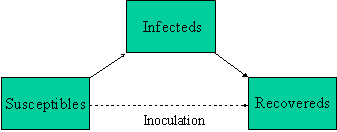
The point of inoculation is to create herd immunity by stimulating in as many people as possible the antibodies that confer immunity -- but without actually giving those people the disease. Thus inoculation creates a direct path from the susceptible group to the recovered group without passing through the infected group (see the diagram below). And a large-scale inoculation program to head off an impending epidemic does this rapidly enough to lower the initial susceptible population to a safe level -- safe enough that if a trace level of infection enters the population, a few people may get sick, but no epidemic will develop.

So, what fraction of the population must be inoculated to obtain herd immunity? Or, put another way, how small must  s₀  be to insure that an epidemic cannot get started? It depends on the contact number.

1. Explain why keeping an epidemic from getting started is the same as keeping  di/dt  negative from  t = 0   on.

2. Write the right-hand side of the infected-fraction differential equation
   
   

   

   
   in factored form. Explain why one factor is always positive and why the sign of other factor depends on the size of  s(t).

3. Explain why  s(t)  is a decreasing function, and thus has its largest value at  t = 0. It follows that, if  di/dt   is negative at time  0,   then it stays negative.

4. Show that

   

   Explain why, if  s₀  is less than  1/c,   then no epidemic can develop.

5. From 1912 to 1928, the contact number for measles in the U.S. was 12.8. If we assume that  c  is still 12.8 and that inoculation is 100% effective -- everyone inoculated obtains immunity from the disease -- what fraction of the population must be inoculated to prevent an epidemic?

6. Suppose the vaccine is only 95% effective. What fraction of the population would have to be inoculated to prevent a measles epidemic?

1. Explain briefly the modeling steps that lead to the SIR model.

2. Given a population and disease combination for which the SIR model is appropriate, what are the possible outcomes when a trace of infection is introduced into the population? How can you tell whether there will be an epidemic?

3. Does "epidemic" mean that almost everyone will get the disease? If so, what keeps the spread of disease going? If not, what causes the epidemic to end before everyone gets sick?

4. How can it happen that a large percentage of a population may get sick during an epidemic even though only a small percentage is sick at any one time?

5. Explain briefly the key idea for finding solutions of an SIR model without finding explicit solution formulas.

6. Describe briefly the meaning and significance of contact number.

7. Describe briefly the meaning and significance of herd immunity. How can an inoculation program lead to herd immunity?

8. The contact number for poliomyelitis in the U.S. in 1955 was 4.9. Explain why we have been able to eradicate this disease even though we cannot eradicate measles. Give a careful argument -- "smaller contact number" is an observation, not an explanation.