In this article we focus on the impact of technology in the teaching and learning of mathematics courses preceding calculus. Our goal is to describe a framework (page 3) that allows instructors and students to explore mathematics in technology-rich settings. To this end we first identify four skill levels for mathematics students:

Antonio Quesada is a Professor of Mathematics at the University of Akron. Michael Todd Edwards is an Assistant Professor of Mathematics and Education at John Carroll University.

• data analysis-based strategies,
• dynamic geometry-based strategies,
• functional model-based strategies,
• calculus-based strategies.

Then we illustrate that technology greatly broadens the group of students who have access to the ideas, by showing how students at all levels can successfully solve the same optimization problem when the appropriate technological tools or other techniques are incorporated.

Published June, 2005

© 2005 by Antonio Quesada and Michael Todd Edwards

Incorporating technology into the teaching and learning of mathematics has impacted various aspects of our instruction, from course content and teaching methodologies to classroom activities and assessment. The use of technology has encouraged us to re-examine our preconceived notions regarding the accessibility of various mathematical topics at various levels of instruction. As Quesada (2000) notes, ''the assumptions many of us made about mathematics curricula in a time prior to graphing calculators are, in many cases, no longer valid.''

Prior to the introduction of technology into mathematics classrooms, the types of problems that a typical student could solve depended largely upon his or her previous coursework. In such settings it was common for Instructors to identify an exercise as a ''precalculus'' problem or an ''advanced algebra'' problem based on the prerequisite mathematics skills required to generate a reasonable solution with pencil and paper.

Many calculus authors and instructors often treat optimization ("max/min") as their own domain, as if it had never been seen anyplace else, and in traditional curricula, such problems were often deferred to calculus. Historically, activities involving optimization, such as the "Two Towers Problem" (TTP) in Figure 1, were considered calculus problems. Because traditional solutions to activities such as the TTP often prompted the use of trigonometry and differential calculus, such problems were considered inaccessible to first-year algebra students using pencil-and-paper techniques.

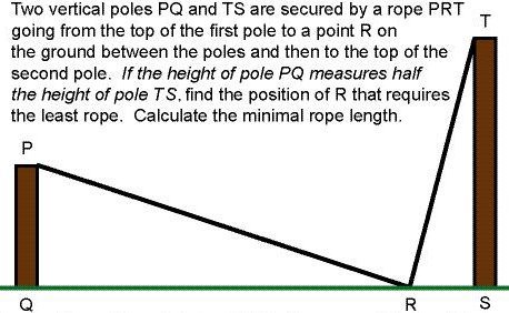
Figure 1. The Two Towers Problem (Source: Adapted from Stewart, 2001 )

As we've introduced technology-based problem-solving tools in our classrooms, the distinctions among activities appropriate for students at various instructional levels have become less clear to us. For instance, students in our developmental courses typically possess little or no knowledge of trigonometry or calculus. Nonetheless, they successfully build models and solve the TTP using dynamic geometry tools (such as Geometer's Sketchpad or Cabri Geometry II). In fact a whole host of optimization problems, traditionally not introduced to students in courses prior to calculus, may now be modeled in this fashion.

Some examples of other easily accessible optimization problems

Clicking and dragging points within their models, our students generate and test conjectures regarding relationships among different variables in their sketches. In the TTP, students look for relationships among lengths (e.g. QR), angle measures (e.g. angles PRQ and TRS), and minimal rope length. As they study algebraic concepts, our students investigate the TTP as a technology-based data analysis activity. After collecting data from physical models, they use calculator-based regression tools to compute ''fit'' equations that describe the relationship of QR to total rope length. In short, students at various levels may use technology meaningfully to explore problems previously constructed for the most advanced mathematics students.

On the next page we describe a framework that may be useful for both instructors and students as they explore mathematics in technology-rich settings. This framework has proved useful for us as we've constructed problems for our students to explore with technology from a variety of perspectives.

Our students have also used the framework to compare the relative advantages and disadvantages of various technology-oriented problem-solving approaches. When our students possess multiple solution strategies for a given problem, the likelihood of their generating mathematically correct solutions is enhanced significantly. In addition, exploring problems from several vantage points encourages our students to build connections among various areas of mathematical study.

Classroom instruction that explicitly explores and compares various solution strategies enhances our students' problem-solving power. Considering that more than half of college math enrollments are at the high school or developmental level, we feel that such explorations are quite relevant for all these students and equally important for pre-service teachers. Although our students use a variety of different tools to solve problems such as the TTP (e.g. Excel, Derive, Mathematica, Maple), in this article we pay particular attention to solutions that use graphing calculators, since their cost and portability make them a popular choice among many high school and college students.

A mathematics program that revisits fundamental problems throughout a student's academic career, while encouraging the use of problem-solving strategies that match his or her current level of conceptual understanding, has the potential to enhance understanding of variable, representation, and mathematical models in a manner not possible with curricular materials that view mathematics as skills obtained in a disjoint collection of courses. This is consistent with the NCTM Problem Solving Standard that suggests that "students be given the opportunity to learn important content through their exploration of the problems and to learn and practice a wide range of heuristic strategies" (NCTM, 2000, p. 341).

Here is a list of general strategies that are available to our students as they solve mathematics problems using technology. For convenience sake, we've divided these strategies into four levels. The levels correspond roughly to courses taken by high school mathematics students or developmental students at the post-secondary level.

• Level 1: Data Analysis-based Strategies (~ introductory algebra)
• Level 2: Dynamic Geometry-based Strategies (~ introductory geometry)
• Level 3: Functional Model-based Strategies (~ advanced algebra or trigonometry)
• Level 4: Calculus-based Strategies (~ precalculus or calculus)

Figure 2 provides a graphical depiction of these strategies.

Figure 2. Strategies for solving mathematics problems with technology

The following aspects of the graphical model are worth examining in greater detail.

Encompassing Scope

A given level within the figure wholly encompasses all levels that precede it. For instance, data analysis and geometry-based strategies (Levels 1 and 2, respectively) lie within Level 3. This suggests that students in our courses who have access to function-model problem-solving strategies may also examine problems from either a geometric or data analysis-based perspective. As our students progress mathematically, they have more choices associated with solution strategies. Recognizing this, we strive to build activities that are accessible to as many of the levels as possible.

Mathematical Rigor

Although it is tempting to consider higher levels to be mathematically more rigorous, this is not necessarily the case. For instance, students using dynamic geometry tools (a Level 2 technique) may ultimately write proofs to generalize their findings. Such an activity may be more "rigorous" than calculator-based regression (a Level 3 approach).

To better describe and elaborate the proposed framework, we examine the TTP from each of the four levels described in Figure 2 .

Level 1: Data Analysis

First, we provide each of our students with a worksheet that models a specific instance of the ''Two Towers'' scenario (e.g., with PQ = 4 cm and QS= 12 cm). Next, we ask our students to draw a point R anywhere along segment QS then estimate total rope length (i.e. PR+RT) using a centimeter ruler. We show a sample worksheet, annotated with student work, in Figure 3.

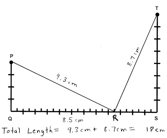
Figure 3. Worksheet modeling the ''Two Towers'' scenario showing student work

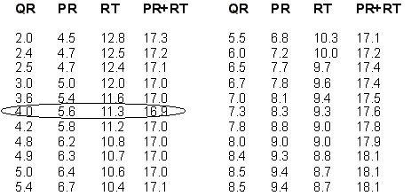
Figure 4. ''Two Towers'' data collected from 22 introductory algebra students

Level 2: Geometric/Dynamic Geometry

A handful of our students are able to solve the TTP without the use of technology -- e.g., by invoking the optical principle of incidence and reflection with straight-edge and compass. However, technology greatly broadens the group of students who have access to the ideas of optimization. Students with previous exposure to dynamic geometry software may perform the data collection in the previous section more precisely. Using software such as CABRI Geometry II (Texas Instruments, 1996) or Geometer's Sketchpad (Key Curriculum Press, 2002), our students examine the relationship of angle PRQ and angle TRS to total rope length without resorting to use of trigonometric functions or even protractors or rulers.

Use of dynamic geometry software has become commonplace in many middle and secondary school classrooms -- in fact, there are free versions of CABRI for TI-83+, TI-92+ and Voyage 200 calculators. With the software, instructors have the ability to create Java-based models of the Two Towers problem that students explore either in class or at home in a web browser. Similarly, students with access to the appropriate software can construct a CABRI model or Sketchpad model of the problem situation.

Unlike a "static" sketch drawn with pencil on a worksheet, a "dynamic" sketch may be modified by clicking and dragging. Measurements of various geometric objects (e.g. segments, angles) are updated automatically as the user moves objects along the screen. In Figure 5, we show a screenshot generated from a dynamic sketch of the Two Towers problem, which illustrates collection of various measures of angle PRQ, angle TRS, and total rope length in CABRI Geometry II. By animating point R within CABRI, our students capture numerous measures of angle PRQ, angle SRT, and total rope length quickly and easily. A CABRI-generated table of the results is shown in Figure 6.

Figure 5. Selecting the Tabulate menu item within CABRI to collect
data regarding measurements that appear within a sketch

After our students select values to tabulate, they drag on point R to animate their sketches. As measures of angle PRQ, angle TRS, and rope length (i.e. PR+RT) change, these values are collected in the table -- see Figure 6.

Figure 6. After the animation, the table of requested measures
is populated with values.

As Figure 6 suggests, the length of the rope appears to be minimal (16.97 units) when angles PRQ and TRS are congruent.

Alternatives to animation and tabulation exist. For instance, once the dynamic model is built, students may use ''trial and error'' to approximate a minimum. Paying careful attention to the value of Tot.Rope, students click and drag on point R until the smallest value of PR+RT is found.

Geometry students may take a more sophisticated approach by reflecting line segments RT and TS over segment QS. In this manner, the original exercise is recast as the problem of finding the shortest path between points P, R, and T'. Figure 7 illustrates an initial construction, and Figure 8 shows a construction in which PR+RT is minimized.

Figure 7. A new model constructed by reflecting RT and TS over QS

When a line segment is used to connect T' (i.e. the reflection of T over QS) with P, triangle PRT' is formed. By the triangle inequality, PR + RT' is greater than or equal to PT', with equality holding when points P, R, and T' are collinear.

Figure 8. The shortest path connecting points P, R, and T' occurs when the
points are collinear, in which case angles PRQ and TRS are congruent.

This reflection argument is equivalent to the argument that some (certainly not all) students see in physics to justify the equality of angles of incidence and reflection. However, even the students who do encounter this idea are likely to see it after having access to dynamic tools in a geometry course.

Level 3: Function Model

Students employing function model strategies have a stronger understanding of function and curve fitting. Students with a background of the Pythagorean Theorem may set up a function that describes the total length of rope. Denoting the horizontal distance between the two poles as w and the height of the poles as n and 2n, total rope length may be expressed as . We illustrate this approach in Figure 9.

Figure 9. Students with knowledge of functions and the Pythagorean Theorem
may express total rope length as a function of QR.

As Figure 10(a) suggests, the algebraic expression for rope length may be typed into the y= editor of a graphing calculator for further examination. Because rope length is defined generally, in terms of parameters n (length of pole PQ) and w (distance between the poles), students may investigate the function for various pole heights and distances by entering values into parameters N and W from the calculator home screen -- see Figure 10(b).

Figure 10. (a) Function for total rope length as it appears in the TI-83+ y= editor;
(b) Students may assign values to parameters N and W with the Store command.

After setting up reasonable display dimensions, students graph the total length function for their selected values of n and w. They can then use the minimization feature of their calculator to find minimal rope length, as illustrated in Figure 11.

Figure 11. (a) Window settings for total rope length function;
(b) Plot of rope length with respect to length of segment QR (i.e. x).
Rope length appears to be minimized when QR = 4 cm.

To provide all students with an opportunity to experience the function analysis, we give different teams or individuals different values of n and w. From their home screens, our students change the values of the parameters and then find the minimum rope length for their particular values. In a class of 20 students, enough data may be collected to look for relationships among n, w, and minimal rope length. In Figure 12, we provide a table of minimal rope lengths for several different (n, w) pairs.

Figure 12. Values of x that minimize rope lengths for several pairs of n and w

As one might suspect, students quickly conjecture that the value of n (i.e., height of the pole PQ) does not affect minimal rope length. Rather, it appears that minimal rope length is precisely w/3 (i.e., one third of the distance between the poles). Using basic trigonometric ratios and the fact that tan x is a 1-1 function on [0, p/2), students recognize that total rope length is minimized when angles PRQ and TRS have the same measure, as illustrated in Figure 13.

Figure 13. Students may use their knowledge of trigonometric functions
to hypothesize that total rope length is minimized
when angles PRQ and TRS have the same measure.

Recent textbooks (e.g., Larson, et al., 1998) use technology to strengthen students' knowledge of families of continuous functions. In addition to "synthetic" models using the Pythagorean Theorem or trigonometric relationships, students may use calculator-based regression with collected data to construct non-linear models. Our students use models such as these to better interpret the data and make predictions as they attempt to find one that suitably describes the collected data. We highlight such an approach on the next page.

Level 4: Calculus

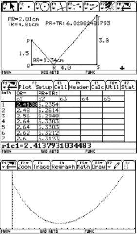Dynamic geometry software has been available on graphing calculators with symbolic manipulation (CAS) capabilities (e.g. TI's Voyage 200) since 1995. With the introduction of CABRI Junior, dynamic geometry software is now available for non-CAS calculators such as the TI-83+. Although the viewscreen of a handheld calculator lacks the larger screen and color capabilities of a desktop computer, investigating problems with calculator-based geometry software provides students with access to the calculator's more powerful, integrated data analysis utilities. Figure 14 illustrates a dynamic sketch and accompanying data analysis using a Voyage 200 calculator.

Once our students generate and collect data using dynamic geometry tools, they study it in detail with the calculator's extensive data analysis utilities. The table in Figure 14 contains 292 points that can be plotted immediately. Constructing a model that fits the plot of total rope length versus QR is not obvious -- it requires significant algebraic thought.

Students who are familiar with calculator-based non-linear regression and who want to avoid a "synthetic" algebraic approach (such as that proposed on the preceding page) may hypothesize that a quadratic or a cubic model will fit the data reasonably well. As Figure 15 illustrates, the relatively large value of the coefficient of determination (R² = 0.989455) and graphical superposition suggest a good fit for a quadratic model.

A cubic model generates a coefficient of determination even closer to 1, namely R² = 0.999367, as illustrated in Figure 16.

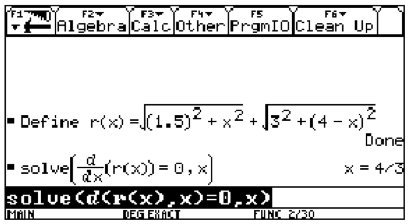
Figure 17. CAS used to calculate critical points for the rope length function r(x)

Our students use the second derivative test in CAS to confirm that a minimum occurs at the critical value -- even though a graph of r(x) would make this evident. By evaluating r(x) at the critical value (in "exact calculation mode"), students calculate minimal rope length exactly, as shown in Figure 18. Note that this closed-form solution contains significantly less information about the problem than either the Level 2 or Level 3 approaches on the preceding two pages.

Figure 18. The second derivative test confirms that a minimum occurs at the
critical value, and the exact value of minimal rope length is calculated.

Up to 30 commands may be stored in the Voyage 200 home screen for review at a later time. Any work session may also be saved as a text file, called a script, that can be recalled, commented, and executed at any time. Students may use a "Two Towers" script as a template to solve similar problems. Hence, a script can be defined as a pseudo-program consisting of a set of commands to accomplish a task (Quesada, 2000). To successfully use a script, the user must provide necessary input and manually execute all template commands one after another.

Non-executable comments may be added to "document" the script. If well-written, the comments describe key goals and steps of the algorithm being performed, thus encouraging the user to review the main ideas of the script each time it is executed. Figure 19 shows a script we've used with our students to automate the calculus-based solution strategy shown in Figures 17 and 18. The use of scripts facilitates the inclusion of new topics and applications, while scaffolding cumbersome calculations that our students have yet to master (Kutzler, 1996). Scripts help our students focus on key algorithmic steps without arithmetic errors and with a minimum investment of time.

Figure 19. "Two Towers" problem script and execution
of the script in the Voyage 200 environment

Alternate approaches

Students may use a power model (which yields no regression coefficient) or a quartic polynomial to fit the data. To compare the relative "goodness of fit" of the models, students calculate the residuals, i.e., the differences between predicted and fitted values for each model. Figure 20 shows the calculation of residuals for power and quartic models.

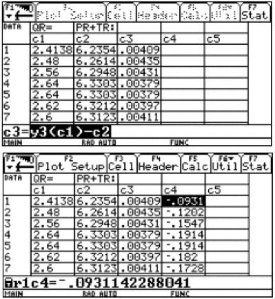
Figure 20. With a power model stored in y1, list c3 is defined as y1(c1)-c2
(i.e., predicted - fitted value). Similarly, with a quartic model stored in y2,
list c4 is defined as y2(c1)-c2.

A cursory examination of residuals for these two models suggests the quartic polynomial produces a better fit than the power model.

The Two Towers Problem is easily generalized in several ways beyond the version found in Stewart.  For example:

• If the ratio of the taller tower to the smaller tower is m, then how does the location of the critical point change as a function of m?
• If the restriction between the poles' heights is removed entirely, show that the critical point is still determined by similarity of the two triangles.

Clearly, all the solutions presented in this article will still apply.

In addition, you or your students may suggest other problem solving avenues, such as equating the slopes of the segments PR and RT'.

Here again is the link from page 2 to other familiar optimization problems that would serve to illustrate various solution techniques that are accessible at each of the four levels of the framework.

Some examples of other easily accessible optimization problems

You may know these problems as

1. the riverbank fence problem,
2. the kite design problem,
3. the isosceles triangle inscribed in circle problem,
4. the ladder over the fence problem.

Through an examination of various technology-based solutions for the Two Towers Problem, we have demonstrated that the incorporation of technology blurs boundaries between various levels of mathematics instruction. Exercises originally conceived for students in advanced courses (such as calculus) may now be explored meaningfully by students in introductory settings. A spiral approach to optimization through different courses preceding calculus has the potential of improving students' understanding of modeling.

Use of dynamic geometry tools, such as CABRI Geometry II and Geometer's Sketchpad, graphing calculators, and mathematical software encourage us to re-examine the accessibility of various mathematical topics. Because technology enables students to revisit problems from different perspectives based upon the depth of their mathematical knowledge, the tools encourage students to make connections among various levels (and areas) of mathematics.

Edwards, M. T. & Reeder, J. (2004). ''Uncovering Unexpected Mathematical Connections with the 'Folded' Triangles Problem.'' Ohio Journal of School Mathematics 49. Columbus, Ohio: Ohio Council of Teachers of Mathematics.

Key Curriculum Press (2002). The Geometer's Sketchpad 4.06 [Computer software]. Berkeley, CA: Key Curriculum Press.

Kutzler, B. (1996). Improving Mathematics Teaching with DERIVE. Lancashire, England, Chartwell-Yourke.

Larson, R., Hostetler, R., & Edwards, B. H. (1998). Calculus (6th edition). Boston, MA: D.C. Heath Company.

National Council of Teachers of Mathematics (2000). Principles and Standards for School Mathematics, Reston, VA: NCTM

Quesada, A. (2000). "The Use of Scripts On Teaching Linear Algebra." Proceedings of the Twelfth Annual International Conference on Technology in Collegiate Mathematics, pp. 329-334, Reading, MA: Addison-Wesley

Stewart, J. (2001). Calculus: Concepts and Contexts (2nd edition). New York: Brooks/Cole

Texas Instruments (1996). Cabri Geometry II, Dallas, TX: Texas Instruments