The Japanese Theorem for Nonconvex Polygons
Abstract. The so-called "Japanese theorem" dates back over 200 years; in its original form it states that given a quadrilateral inscribed in a circle, the sum of the inradii of the two triangles formed by the addition of a diagonal does not depend on the choice of diagonal. Later it was shown that this invariance holds for any cyclic polygon that is triangulated by diagonals. In this article we examine this theorem closely, discuss some of its consequences, and generalize it further. In particular, we explore its relationship with Carnot's classical theorem on triangles, we look for extreme values for this sum of inradii, we look at the limit of this value as the number of sides goes to infinity, and we generalize the theorem to nonconvex cyclic polygons. We include interactive applets throughout the article to give the theorems a tangible credibility.
The Japanese Theorem for Nonconvex Polygons - A Japanese Temple Problem
A Japanese Temple Problem
In 1800, Ryōkwan Maruyama inscribed a geometry problem onto a wooden tablet and hung it in the Tsuruoka-Sannōsha shrine in what was then the Uzen Province in the northern part of Japan's Honshu island ([AUM3, Hay]). While posting a mathematical puzzler in a Shinto shrine sounds strange to us today, it was not uncommon at that time in Japan.
Japan was completely closed off from the outside world for almost the entire Edo period (1603–1868) in which Japan was ruled by the Tokugawa shogunate. Almost nothing penetrated the enforced isolation of the country, not even mathematical ideas such as the calculus of Newton, Leibniz, and Euler.
However, during this time the Japanese continued to study mathematics, or wasan, as it was called. There developed a curious tradition of inscribing geometry problems, complete with elegant and colorful figures, on wooden boards and posting them in Shinto shrines and Buddhist temples. They were gifts to the gods as well as mathematical challenges to the visitors. The boards were known as sangaku, which means "mathematical tablet." Approximately 900 sangaku survive today, but it is believed that thousands more have been lost. For more information about sangaku see [FP] or [FR].
Maruyama's sangaku is one of those that disappeared, but fortunately the inscription was recorded in the second volume of Kagen Fujita's 1807 Zoku-Sinpeki-Sanpō ([AUM3, Fu]). As was tradition, Maruyama also included the answer to the problem and a brief description of how to arrive at this answer, called the art of the problem. But he included no proof. According to [Fu] the inscription read:
Problem: draw six lines in the circle and make four circles inscribed in three of the lines. If the diameter of the southern, eastern, and western circle is 1 sun [a traditional Japanese unit of measure which is approximately 1.19 inches], 2 suns, and 3 suns, respectively, how long is the diameter of the northern circle?
Answer: 4 suns.
Art: Add the diameter of the western circle to that of the eastern one and subtract that of the southern one from it, and you will get that of the northern one. End.
 Figure 1
According to [FP], the first known proof of this sangaku problem is found in the undated manuscript [Yo].
The Japanese Theorem for Nonconvex Polygons - The Japanese Theorem for Quadrilaterals
The Japanese Theorem for Quadrilaterals
The art of Maruyama's sangaku problem implies that in any such configuration \(d_N = d_E + d_W - d_S\), where \(d_N, d_E, d_W\), and \(d_S\) are the diameters of the northern, eastern, western, and southern circles, respectively. Equivalently, using radii,
\[r_N + r_S = r_E + r_W.\]
This surprising result is now known as the Japanese theorem.
The Japanese theorem for quadrilaterals. Add a diagonal to a convex quadrilateral whose vertices lie on a circle. Inscribe circles in the resulting triangles. The sum of the radii of the inscribed circles does not depend on the choice of diagonal.
Below we have an applet illustrating this invariance. The circle has radius 1. Move the points around the circle and observe that the sum of the radii of the red circles equals the sum of the radii of the blue circles. There is an additional fascinating fact about this construction that we will not pursue: the centers of the four circles form a rectangle ([p. 255, Jo1]).
In this article we examine this extremely beautiful theorem. We not only prove the theorem, but we also endeavor to illustrate why the theorem is true. We explore some consequences of the theorem, and we generalize it further to polygons with intersecting sides.
The Japanese Theorem for Nonconvex Polygons - First Generalizations
First Generalizations
Just after the turn of the twentieth century the Japanese mathematician Yoshio Mikami heard of a theorem from a friend, who had heard it from someone from China. No proof accompanied the theorem. In 1905 Mikami stated and proved the theorem ([Mi]):
If in a polygon inscribed in a circle all possible diagonals that can be drawn from a vertex are drawn and the successive triangles thus formed are inscribed with circles, then their radii will be together equal for any of the vertices.
For example, the polygon in Figure 2 is triangulated with diagonals meeting at two different vertices, but the sums of the radii are equal.
 Figure 2
This remarkable theorem immediately got the attention of other Japanese mathematicians and new proofs appeared in print the following year—one in [Gr] and five compiled in [Hay]. In this latter paper, the author points out that this "soi-disant théorème Chinois" (so-called Chinese theorem) is simply a generalization of Maruyama's hundred-year-old sangaku problem and could be established from it using induction. Moreover, Fujita's books were commonly used in schools, so he contends that the theorem's Chinese origin is "douleuse" (doubtful).
This theorem received its widest exposure when it appeared in Roger Johnson's 1929 classic text Modern Geometry ([p. 193, Jo1]), which was reprinted by Dover in 1960 as Advanced Euclidean Geometry ([Jo2]).
In 1985 Ross Honsberger observed that there are many other ways to triangulate an \(n\)-gon with nonintersecting diagonals (the number of ways is precisely the \( (n-2)\)nd Catalan number) and that invariance holds in these situations as well ([p. 24, Ho]):
A great deal more might have been claimed [by Johnson], for this same sum results for every [author's emphasis] way of triangulating the polygon!
 Figure 3
We call this the Japanese theorem for polygons.
The Japanese Theorem for Nonconvex Polygons - The Japanese Theorem for Polygons
The Japanese Theorem for Polygons
A cyclic polygon is a polygon all of whose vertices lie on a circle (for now we assume that the polygon is convex; that is, the edges do not cross). The inradius and circumradius of a triangle are the radii of the inscribed and circumscribed circles, respectively. The theorem stated and proved by Honsberger is the following.
The Japanese theorem for polygons. Triangulate a convex cyclic polygon using nonintersecting diagonals. The sum of the inradii of the triangles is independent of the choice of triangulation.
Let \(P\)
The following applet gives three different triangulations of a cyclic polygon. Move the vertices to see that the sums remain the same.
Remark: if the polygon is not cyclic then the total inradius is not independent of triangulation. In 1994 Lambert ([L]) proved that in general the largest total inradius is achieved by the Delaunay triangulation, which is the planar dual to the well-known Voronoi diagram.
The Japanese Theorem for Nonconvex Polygons - Carnot's Theorem
Carnot's Theorem
For proofs of the quadrilateral case of the Japanese theorem or the polygonal case with all diagonals eminating from a single vertex see [AUM1, AUM2, FP, FR, Gr, Hay, Jo1, Mi, Yo]. We will not prove those separately, but instead prove the more general Japanese theorem for cyclic polygons. Our proof, which is in essence Honsberger's proof ([Ho]), relies on a classical theorem discovered by Lazare Nicolas Marguérite Carnot (1753–1823) that exhibits a relationship between a triangle, its inradius, and its circumradius.
The signed distance of a side of a convex cyclic polygon to the circumcenter is the distance, unless the segment joining the cirucumcenter to the side lies completely outside the polygon, in which case it is the negative of the distance. For example, for the triangles in Figures 4(a) and 4(b), all the signed distances \(a, b,\) and \(c\) are positive except \(b\) in Figure 4(b). The sign contributions of the cyclic hexagon in Figure 4(c) are indicated.
 Figure 4
Carnot's theorem. If \(a\), \(b\), and \(c\) are the signed distances from the circumcenter of a triangle to the sides of the triangle, \(R\) is the circumradius, and \(r\) is the inradius, then \(R + r = a + b + c\).
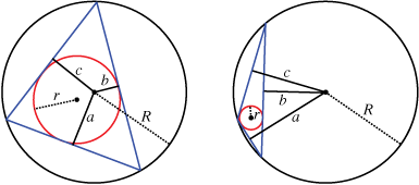 Figure 5
See [AN] for a short proof of Carnot's theorem for acute triangles (in this case \(a\), \(b\), and \(c\) are all positive); the given argument can be modified to cover the non-acute case.
To see the theorem in action, move the vertices of the triangle below and see the equality of the two sums.
The Japanese Theorem for Nonconvex Polygons - Carnot's Theorem for Cyclic Polygons
Carnot's Theorem for Cyclic Polygons
In order to prove the Japanese theorem we need to generalize Carnot's theorem to cyclic polygons.
Carnot's theorem for cyclic polygons. Suppose \(P\) is a cyclic \(n\)-gon triangulated by diagonals. Let \(R\) be the circumradius of \(P\), let \(d_1, d_2, \cdots, d_n\) be the signed distances from the sides of \(P\) to the circumcenter, and let \(r_1, r_2, \cdots, r_{n-2}\) be the inradii of the triangles in the triangulation. Then
\[(n-2)R + \sum_{k=1}^{n-2} r_k = \sum_{i=1}^n d_i .\]
Proof. This is a proof by induction. The base case, \(n=3\), is simply Carnot's theorem for triangles. Now suppose the theorem holds for some \(n \geq 3\). Let \(P\) be a cyclic \((n+1)\)-gon that is triangulated by diagonals. Because the triangulation has \(n - 1\) triangles, the pigeonhole principle tells us that there is a triangle that has two edges in common with \(P\). Without loss of generality, the signed distances to these two shared edges are \(d_n\) and \(d_{n+1}\), and the inradius of this triangle is \(r_{n-1}\). Remove this triangle to obtain a cyclic \(n\)-gon \(P'\) and let \(d_n^{\prime}\) be the signed distance to the new edge. By the induction hypothesis
\[\sum_{k=1}^{n-2} r_k = (2-n)R + d_n^{\prime} + \sum_{i=1}^{n-1} d_i .\]
Now consider the removed triangle. The key observation is that the signed distances from the circumcenter to the sides of the triangle are \(-d_n^{\prime}\), \(d_n\), and \(d_{n+1}\). (For example, in Figure 6(a) the dashed edge is positive when viewed as a side of triangle \(p_1p_4p_5\), but negative when viewed as a side of polygon \(p_1p_2p_3p_4\), and similarly in Figure 6(b) the dashed edge is negative when viewed as a side of triangle \(p_1p_4p_5\), but positive when viewed as a side of polygon \(p_1p_2p_3p_4 .\))
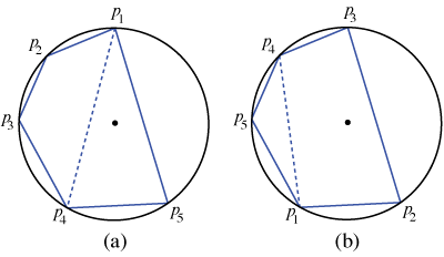 Figure 6
By Carnot's Theorem for triangles \(r_{n-1} + R = -d_n^{\prime} +d_n +d_{n+1}\). Consequently,
\(\sum_{k=1}^n r_k = (\sum_{k=1}^{n-2} r_k) + r_{n-1}\)
\(= ((2-n)R + d_n^{\prime} + \sum_{i=1}^{n-1} d_i) + (-R + (-d_n^{\prime} + d_n + d_{n+1}))\)
\(= (2-(n+1))R + \sum_{i=1}^{n+1} d_i .\)
as was to be shown.∎
The Japanese theorem follows immediately from this version of Carnot's theorem.
Proof of the Japanese Theorem. Let \(P\) be an \(n\)-gon inscribed in a circle of radius \(R\) . Carnot's theorem for cyclic polygons says that for any triangulation of \(P\) by diagonals
\[r_P = \sum_{k=1}^{n-2} r_k = (2-n)R + \sum_{i=1}^n d_i ,\]
where \(r_k\) and \(d_i\) are defined as above. But \(R, n\) and the \(d_i\) do not depend on the choice of triangulation, so the total inradius, \(r_P\), does not either.∎
These results provide an interesting way of seeing what \(r_P\) measures. Rearranging terms we obtain
\[r_P = 2R - \sum_{k=1}^n (R - d_k) .\]
The quantity \(R - d_k\) is the amount that the perpendicular drawn to the \(k\)th side of \(P\) differs from the radius of the circumcircle. So \(r_P\) is the diameter of the circle minus the sum of these differences. Thus, larger values of \(r_P\) correspond to polygons that more closely approximate the circle. Later we show that by increasing the number of sides we can find a polygon with a total inradius as close to \(2R\) as we please.
The Japanese Theorem for Nonconvex Polygons - The Space of Cyclic Polygons
The Space of Cyclic Polygons
The Japanese theorem tells us that we may associate a single numerical value, \(r_P\), to each cyclic polygon \(P\). In other words, we have found a real-valued function on the space of cyclic polygons. Let us explore this idea a little further.
For simplicity, assume that all of our polygons are inscribed in a circle of fixed radius \(R\) with its center at the origin. We denote the space of cyclic \(n\)-gons \(\mathcal{P}_{R,n}^c = \mathcal{P}_n^c\) (the superscript \(c\) refers to the fact that these are convex polygons, we'll consider nonconvex ones later) and define the function \(f:\mathcal{P}_n^c \rightarrow \mathbb{R}\) to be \(f(P) = r_P\).
Let us be more precise about our definition of \(\mathcal{P}_n^c\)
We identify each polygon in \(\mathcal{P}_n^c\) with the vector of central angles \(\theta_1, \ldots, \theta_n \) as in Figure 7. That is, if \(p_k = (R \cos (\alpha_k), R \sin (\alpha_k))\), then \(\theta_k = \alpha_{k+1} - \alpha_k \) for \(k = 1, \ldots, n-1\) and \(\theta_n = 2 \pi - \alpha_n .\) In this way, we may express
\[\mathcal{P}_n^c = \{(\theta_1, \ldots, \theta_n) \in [0, 2 \pi]^n: \theta_1+ \cdots + \theta_n = 2 \pi\}.\]
If we want to exclude the degenerate polygons, then we insist that \(\theta_k > 0\) for all \(k\).
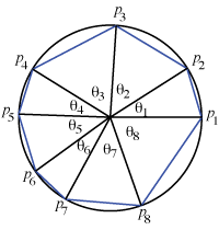 Figure 7
Thus the space of cyclic \(n\)-gons is an \((n-1)\)-dimensional simplex with the interior of the simplex corresponding to the nondegenerate polygons. For example the space of cyclic triangles is an equilateral triangle and the space of cyclic quadrilaterals is a tetrahedron. A vertex of this simplex corresponds to the degenerate polygon for which \(p_1 = \cdots = p_n\); we can safely ignore the fact that these \(n\) points, \((2 \pi, 0, \ldots, 0), (0, 2 \pi, 0, \ldots, 0), \ldots, (0,\ldots, 0, 2 \pi) ,\) all correspond to the same polygon. Similarly, an edge corresponds to \(n - 1\) vertices equal and one different, and, in general, a \(k\)-dimensional facet corresponds to \(\{ p_1, \ldots, p_n\} \) being \(k + 1\) distinct points on the circumcircle.
The Japanese Theorem for Nonconvex Polygons - The Total Inradius Function
The Total Inradius Function
Using the notation given on the previous page, elementary trigonometry, and the polygonal Carnot's theorem we are able to give an explicit formula for the function \(f: \mathcal{P}_n^c = \mathcal{P}_{R,n}^c \rightarrow {\mathbb R} .\)
Let \(P \in \mathcal{P}_n^c .\) By the polygonal Carnot's theorem,
\[f(P) = r_P = (2-n)R + \sum_{k=1}^n d_k\]
where \(d_k\) is the signed distance from the center of the circle to the \(k\)th side of the polygon. Notice that \(d_k > 0\) precisely when \(\theta_k < \pi .\) In particular, as we see in Figure 8, \(d_k = R \cos( \theta_k/2) .\) When \(\theta_k \geq \pi , \) \(d_k = -R \cos (\pi - \theta_k / 2) = R \cos( \theta_k / 2) ,\) as well.

Figure 8
Thus, we obtain the following explicit expression for the total inradius function in terms of \(\theta_1 , \ldots , \theta_n :\)
The Japanese Theorem for Nonconvex Polygons - Extreme Values for the Radial Sum Function
Extreme Values for the Radial Sum Function
Now that we have a formula for the total inradius function we can look for extreme values of the function; in other words we can determine which polygons yield the largest and smallest total inradius.
Theorem. Let \(\mathcal{P}_n^c = \mathcal{P}_{R,n}^c\) be the space of convex cyclic \(n\)-gons with circumradius \(R\), and let \(f: \mathcal{P}_n^c \rightarrow {\mathbb R}\) be the function given by \(f(P) = r_P .\)
1. The unique absolute maximum of \(f\) is the regular \(n\)-gon \(P_n .\)
2. The set of absolute minima of \(f\) is the 1-skeleton of \( \mathcal{P}_n^c .\)
3. The function \(f\) has no relative, non-absolute extrema.
Proof. From the definition of \( \mathcal{P}_n^c\) and the representation of \(f\) given on the previous page, it suffices to investigate the extrema of the function
\[f(P) = f(\theta_1, \ldots, \theta_n) = R \left( 2 - n + \sum_{k=1}^n \cos\left(\frac{\theta_k}{2} \right) \right) \]
subject to the constraints \( g ( \theta_1, \ldots, \theta_n) = 2 \pi\) and \(\theta_k \geq 0 .\) By the method of Lagrange multipliers, extreme values occur when \( \nabla f = \lambda \nabla g \) for some constant \(\lambda\) or when \( (\theta_1, \ldots, \theta_n) \) is on the boundary of the simplex \( \mathcal{P}_n^c .\)
Observe that \( \nabla f = ( -R \sin (\theta_1 / 2)/2, \ldots, -R \sin(\theta_n / 2)/2)\) and \( \nabla g = (1, \ldots, 1) .\) Thus, interior extrema can only occur when \( \sin(\theta_1 /2) = \cdots = \sin(\theta_n / 2) \) and \( \theta_1 + \cdots + \theta_n = 2 \pi .\) Clearly \( \theta_1 = \cdots = \theta_n =2\pi/n \) is one such point (this is the regular \(n\)-gon \( P_n\)). In this case \( f(P_n) = R(2-n(1 - \cos(\pi / n))) .\) We claim that there are no other extreme values in the interior of the simplex and that this is the absolute maximum.
Suppose that \( (\theta_1, \ldots, \theta_n) \)
The Japanese Theorem for Nonconvex Polygons - Regular Polygons
Regular Polygons
In our previous theorem we saw that for a fixed \(n\) and fixed \(R\) the maximum value of \(r_P\) is attained by the regular \(n\)-gon, \(P_n\). Thus we may ask, how large can \(r_P\) get for all \(n\)?
Theorem. If \(P_n\) is a regular \(n\)-gon inscribed in a circle of radius \(R\), then \((r_P)_{n=3}^{\infty}\)
We illustrate this theorem using the applet below. The \(n\)-gons are inscribed in a circle of radius 1. Use the slider to increase the number of sides of the polygon and observe the value \(r_{P_n}\)
Proof. By our previous theorem, the radial sum of the regular polygon \(r_{P_n}\) is
\[r_{P_n} = R \left(2 - n + \sum_{k=1}^n \cos \left( \frac{\theta_k}{2} \right) \right) = R \left( 2 - n + n \cos \left( \frac{\pi}{n} \right)\right) . \]
It is straightforward to show that this is an increasing function of \(n\) when \(n > 2\). Moveover, by a change of variables and an application of l'Hospital's rule we have
\[\lim_{n \rightarrow \infty} r_{P_n} = \lim_{n \rightarrow \infty} R \left(2 + n \left( \cos \left( \frac{\pi}{n} \right) - 1 \right) \right) \]
\[ = R \left( 2 + \lim_{m \rightarrow 0^+} \frac{\cos(m \pi) - 1}{m} \right)\]
\[ = R \left( 2 + \lim_{m \rightarrow 0^+} - \pi \sin(m \pi) \right)\]
\(=2 R .\)∎
\[r_P = 2R - \sum_{k=1}^n (R - d_k) .\]
For regular polygons this implies that \(r_{P_n} = 2R - n(R - D_n) , \) where \(D_n\) is the distance from the center of the circle to a side of the regular \(n\)-gon \(P_n\). This theorem says that \(D_n\) approaches \(R\) fast enough that the term \(n (R - D_n)\) goes to zero.
Although the proof and the applet show that the total inradius tends toward the diameter, it may not be apparent why this is so. In Figure 9 we see that this result is more clear if we choose a different triangulation.

Figure 9
The Japanese Theorem for Nonconvex Polygons - Limiting Behavior
Limiting Behavior
We have seen that the total inradii of regular polygons tend to the diameter of the circle. We now prove a slightly different theorem on the limiting behavior of cyclic polygons.
Theorem. Let \(A = \{ a_k : k \in {\mathbb Z}^+ , a_i \neq a_j \) for \( i \neq j\} \)
We leave the proof of the following lemma to the reader.
Lemma. \( \cos (x) + \cos (y) \geq \cos(x+y) + 1 \) for any \( (x,y) \) in the region bounded by \( x = 0, y = 0, \) and \( x + y = \pi , \) with equality only on the boundary.
Proof of theorem. Because \(A\) is dense, there is an \(M\)
\[ r_{P(n+1)} = R \left( 2 - (n+1) + \sum_{k=1}^{n+1} \cos \left( \frac{\theta_k}{2} \right) \right) \]
and
\[ r_{P(n)} = R \left( 2 - n + \sum_{k=1}^{n-1} \cos \left( \frac{\theta_k}{2} \right) + \cos \left( \frac{\theta_n + \theta_{n+1}}{2} \right) \right) . \]
From the preceding lemma it follows that \( r_{P(n)} < r_{P(n+1)} . \) So the sequence \( \left( r_{P(n)} \right)_{n=3}^{\infty} \) is eventually increasing.
By our theorem on regular polgyons we know that for a given number of vertices, the largest radial sum is obtained from the regular \(n\)-gon and this value is bounded above by \(2R .\) Consequently, the sequence \( \left( r_{P(n)} \right) \) is eventually increasing and is bounded above by \( 2R .\) Thus, to prove the theorem it suffices to show that for a given \( \epsilon > 0 , \) there exists an \(N\) such that \( r_{P(N)} > 2R - \epsilon .\) By the limiting theorem for regular polygons there exists an \( m > 4 \) such that \( r_{P_m} > 2R - \epsilon / 2 , \) where \( P_m \) is a regular \(m\)-gon. Since \(A\) is a dense set, there exist \(m\) distinct points \(A^{\prime} = \{ a_{n_1}, a_{n_2}, \ldots, a_{n_m} \} \subset A\) close enough to the \(m\) vertices of \( P_m \) that the polygon \( P^{\prime} \) with vertex set \( A^{\prime} \) has \( r_{P^{\prime}} > 2R - \epsilon \).∎
The Japanese Theorem for Nonconvex Polygons - Irrational Rotations of the Circle
Irrational Rotations of the Circle
We now illustrate the previous theorem with a concrete example. Recall the following well-known theorem (see [p.53,R], for instance).
Theorem. If \(\alpha \) is a irrational number, then the sequence \( \left( \left( \cos(2 k \pi \alpha), \sin(2 k \pi \alpha) \right) \right)_{k=0}^{\infty} \) is a dense subset of the unit circle.
This theorem says that if we take the point \( (1,0) \) and repeatedly rotate it by an angle \(2 \pi \alpha \) about the origin, then the orbit will be dense in the circle. Note that if \( \alpha = p/q \) is rational and is expressed in lowest terms with \( q > 0 ,\) then the orbit consists of \(q\) points.
Use the applet below to see the sequence of total inradii for various irrational values of \( \alpha . \)
The Japanese Theorem for Nonconvex Polygons - The Generalized Japanese Theorem
The Generalized Japanese Theorem
When playing with the two applets illustrating the Japanese theorem (for quadrilaterals and for \(n\)-gons), there is a strong temptation to move one vertex past another and make a polygon with crossed edges (as in Figure 10, in which we slide \(p_8\) past \(p_1 \)
 Figure 10
In this section we generalize the Japanese theorem to nonconvex polygons. In order to do so we must reexamine our definitions. We begin with a collection of points on the circle, \( p_1, \ldots, p_n \)
To define triangulation for a nonconvex polygon we must borrow some terminology from graph theory. Recall that a graph is planar if there exists an embedding of the graph in the plane such that no edges cross. A nonconvex polygon is triangulated by diagonals if there is a planar embedding of the \(n\)-gon and \(n - 2\) diagonals such that the polygon is an exterior boundary and all diagonals are nonintersecting. As with convex polygons, an easy way to obtain a triangulation is to pick one vertex and draw diagonals to all the non-neighboring vertices.
As before, we can inscribe a circle in each triangular region and measure the inradius. Now, however, we assign a sign to the inradius. If a triangle has vertices \(p_i, p_j, p_k \) with \(i < j < k\) and \(p_i, p_j, p_k \) are situated around the circle in a counterclockwise fashion, then we say that the triangle is positively oriented, and we take the signed inradius to be the inradius. Otherwise the triangle is negatively oriented, and the signed inradius is the negative of the inradius. For example, in the figure above the triangle with vertices \(p_1, p_5, \) and \(p_8\)
Generalized Japanese theorem. Triangulate a cyclic polygon using diagonals. The sum of the signed inradii of the triangles is independent of the choice of triangulation.
Use the following applet to see the invariance of the total signed inradius, which we denote \( \tilde{r_P} .\)
The proof of this version of the Japanese theorem requires a further generalization of Carnot's theorem.
The Japanese Theorem for Nonconvex Polygons - A Further Generalization of Carnot's Theorem
A Further Generalization of Carnot's Theorem
When we introduced Carnot's theorem we gave a technique for computing the signed distance of a side of a polygon to the circumcenter. We must now generalize this to oriented triangles and more generally to nonconvex polygons.
Suppose we have a cyclic polygon with vertices \( p_1, \ldots, p_n . \) We now define \(d_i\), the signed distance from the \(i\)
In Figure 11 we see three different cyclic polygons with the signs of the \( d_i \) labeled. Notice that the positively oriented triangle in Figure 11(a) corresponds to the original definition.
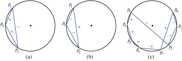 Figure 11
Carnot's theorem for oriented triangles. Let \( T \) be an oriented triangle with circumradius \( R \) and inradius \( r . \) Suppose \( a, b, \) and \( c \) are the signed distances from the circumcenter of \( T \) to the sides of \( T \) and that \( \tilde{r} \) is the signed inradius. If \( T \) is positively oriented, then \( R + r = R + \tilde{r} = a + b + c . \) If \( T \) is negatively oriented, then \( - R - r = - R + \tilde{r} = a + b + c . \)
Proof. If \( T \) is positively oriented, then this is simply the usual Carnot's theorem. Suppose \( T \) is negatively oriented. The signed distances to the sides are the negatives of what they would have been had the triangle been positively oriented. Thus, by Carnot's theorem \( R + r = - a - b - c , \) and by definition \( \tilde{r} = - r . \)∎
Generalized Carnot's theorem for cyclic polygons. Suppose \( P \) is a cyclic \( n \)-gon that is triangulated by diagonals. Let \( d_1, \ldots, d_n \) be the signed distances from the sides of \( P \) to the circumcenter and let \( d_1, \ldots, d_n \) be the signed inradii of the triangles in the triangulation. Suppose there are \( p \) triangles that are positively oriented and \( q \) that are negatively oriented. Then
\[ R ( p - q ) + \sum_{k=1}^{n-2} \tilde{r_k} = \sum_{i=1}^n d_i . \]
Proof. This is a proof by induction on the number of vertices. We may assume they are all distinct; if not, . The base case, \( n = 3 \) is simply Carnot's theorem for oriented triangles. Now suppose the theorem holds for all \( 3 \leq i \leq n \) for some \( n . \) Let \( P \) be a cyclic \( (n+1) \)-gon that is triangulated by diagonals. Furthermore, suppose it has \( p \) triangles that are positively oriented and \( q \) that are negatively oriented. By the pigeonhole principle there is a triangle that has two edges in common with \( P . \) Without loss of generality, we may assume that this triangle has vertices \( p_1, p_n \) and \( p_{n+1} , \) that the signed distances to the two edges shared with \(P\) are \(d_n , \) and \( d_{n + 1} , \) and that the signed inradius of this triangle is \( \tilde r_{n-1} . \) Remove this triangle to obtain a cyclic \( n \)-gon \( P^{\prime} . \) The key fact is that the sign of the signed distance to the newly created side (which has endpoints \( p_1 \) and \( p_n \) is different if viewed as an edge of \( P^{\prime} \) and as an edge of the triangle. (For example, in Figure 12 the sign is positive if viewed as a side of \( P^{\prime} \) and negative if viewed as a side of the triangle.) Let \( d_n^{\prime} \) be the signed distance to this side of \(P^{\prime}\) and \( -d_n^{\prime} \) be the signed distance to this side of the triangle.
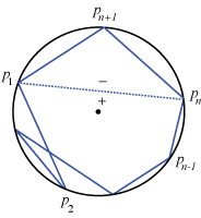 Figure 12
Case 1: the removed triangle is positively oriented. By the induction hypothesis
\[ \sum_{k=1}^{n-2} \tilde{r_k} = R ( q - p + 1) + d_n^{\prime} + \sum_{i=1}^{n-1} d_i . \]
Now consider the removed triangle. By Carnot's theorem for oriented triangles, \( R + \tilde{r}_{n-1} = - d_n^{\prime} + d_n + d_{n+1} . \) Consequently,
\(\sum_{k=1}^{n-1} \tilde{r_k} = \left( \sum_{k=1}^{n-2} \tilde{r_k} \right) + \tilde{r}_{n-1} \)
\( = \left( R ( q - p + 1) + d_n^{\prime} + \sum_{i=1}^{n-1} d_i \right) + ( - R + (- d_n^{\prime} + d_n + d_{n+1})) \)
\( = R(q-p) + \sum_{i=1}^{n+1} d_i , \)
as was to be shown.
Case 2: the triangle is negatively oriented. This case proceeds similarly, except that the induction hypothesis gives
\[ \sum_{k=1}^{n-2} \tilde{r_k} = R(q - 1 - p) + d_n^{\prime} + \sum_{i=1}^{n-1} d_i \]
and for the removed triangle \( - R + \tilde{r}_{n-1} = -d_n^{\prime} + d_n + d_{n+1} . \)
Case 3: the triangle is degenerate. In this case two or three of the vertices \( p_1, p_n , \) and \( p_{n+1} \) coincide. Because \( \tilde{r}_{n-1} = 0 , \) our induction hypothesis gives us
\[ \sum_{k=1}^{n-1} \tilde{r}_k = \sum_{k=1}^{n-2} \tilde{r}_k = R (q - p ) + d_n^{\prime} + \sum_{i=1}^{n-1} d_i . \]
We now consider three subcases. (a) Suppose \( p_1 = p_{n+1} . \) Then \( d_{n+1} = 0 \) and \(d_n = d_n^{\prime} . \) So \( d_n^{\prime} = d_n + d_{n+1} . \) Substituting this into the formula yields the desired conclusion. (b) The case \( p_n = p_{n+1} \) is similar. (c) Suppose \( p_1 = p_n . \) Then \( d_n^{\prime} = 0\) and \(d_n + d_{n+1} = 0 . \) Thus, the result follows.∎
The Japanese Theorem for Nonconvex Polygons - A Proof of the Generalized Japanese Theorem
A Proof of the Generalized Japanese Theorem
Lemma. Given any cyclic polygon, the difference between the number of positively oriented triangles and the number of negatively oriented triangles is independent of the choice of triangulation by diagonals.
Proof. First we will show that the result is true for cyclic quadrilaterals (for which there are two choices for the one and only diagonal). For nondegenerate quadrilaterals there are, up to permutation, three configurations to check—the points are arranged in a clockwise, counterclockwise, or criss-cross pattern. In all of these cases the number of positively and the number of negatively oriented triangles does not change, thus neither does the difference. We've illustrated two of the three cases in Figure 13. In Figure 13(a) both triangulations have two negatively oriented triangles and in Figure 13(b) both have one triangle of each orientation.
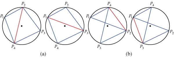 Figure 13
We must also consider degenerate quadrilaterals—those which have three or fewer vertices.The one and two vertex cases have no nontrivial triangles, so we need only consider the three vertex case. There are four such configurations—two that are triangles and two that are vee-shaped. Two of the cases are shown in Figure 14 (the coincidental points are shown slightly separated for illustration purposes). Figure 14(a) has one degenerate triangle and one positively oriented triangle with both choices of diagonal. Figure 14(b) has a positively and a negatively oriented triangle with one diagonal and two degenerate triangles with the other diagonal. Thus, in these cases, and in the other two that are not pictured, the difference is invariant.
 Figure 14
If we have a triangulated cyclic \(n\)-gon and we remove any diagonal, then it leaves an untriangulated quadrilateral. We can then add the other diagonal, which, as we have just shown, does not change the difference in the numbers of positively and negatively oriented triangles. Since it is possible to transform any triangulation into any other triangulation by using this technique repeatedly, the difference is an invariant.∎
Proof of the Generalized Japanese Theorem. By the generalized Carnot's theorem for cyclic polygons
\[ \sum_{k=1}^{n-2} \tilde{r}_k = R(q - p) + \sum_{i=1}^n d_i . \]
Clearly \(R\) and the \( d_i \) are independent of the triangulation, and by the previous lemma, so is \( q - p . \) Thus, so is the left-hand side.∎
The Japanese Theorem for Nonconvex Polygons - Extreme Values for Cyclic Polygons
Extreme Values for Cyclic Polygons
We conclude by looking for extreme values of the total (signed) inradius for cyclic \(n\)-gons. To do so we must look closer at the space of cyclic \(n\)-gons inscribed in a circle of radius \(R\), which we denote \( \mathcal{P}_{R,n} = \mathcal{P}_n \), and the function \( f : \mathcal{P}_n \rightarrow {\mathbb R} \), given by \( f(P) = \tilde{r}_P . \)
As we did for convex cyclic \(n\)-gons, we assume that \(p_1 = (R,0) \) and we identify each polygon in \( \mathcal{P}_n \) with the vector of central angles \( (\theta_1, \ldots, \theta_n ) \), but now the \( \theta_i \) can take on any value; they can even be negative. So, perhaps the most simple representation is
\[ \mathcal{P}_n = \{ (\theta_1, \ldots, \theta_n) \in {\mathbb R}^n : \theta_1 + \cdots + \theta_n = 2 k \pi \text{ for some } k \in {\mathbb Z}
\} , \]
but this representation hides the fact that different \(n\)-tuples can correspond to the same polygon. For instance, \((\theta_1, \ldots, \theta_{n-1}) \text{ and } (\theta_1, \ldots, \theta_{n-1}, 2 \pi + \theta_n ) \) represent the same polygon. Specifically, we have an equivalence relation \( \sim \) in which \( (\theta_1, \ldots, \theta_n) \sim (\theta_1^{\prime}, \ldots, \theta_n^{\prime}) \) provided \( (\theta_1, \ldots, \theta_n) - (\theta_1^{\prime}, \ldots, \theta_n^{\prime}) = (k_1 2 \pi, \ldots, k_n 2 \pi) \) for some \(k_1, \ldots, k_n \in {\mathbb Z} . \) So
\[ \mathcal{P}_n = \{ (\theta_1, \ldots, \theta_n) \in {\mathbb R}^n : \theta_1 + \cdots + \theta_n = 2 k \pi \text{ for some } k \in {\mathbb Z} \} / \sim . \]
Let us simplify this even more. First of all, we may assume that the angles are between \(0\) and \( 2 \pi .\) Then we only have ambiguity at the endpoints. Second, we observe that the \(n\)th coordinate is superfluous since it is uniquely determined by the first \(n-1\) coordinates. So,
\( \mathcal{P}_n = \{ (\theta_1, \ldots, \theta_{n-1}) : 0 \leq \theta_i \leq 2 \pi \} / \sim \)
\( = [0, 2 \pi]^{n-1}/ \sim . \)
This last representation gives us the best way to view \( \mathcal{P}_n . \) The space is the \( (n-1) \)-dimensional cube \( [0, 2 \pi]^{n-1} \) with the opposite faces glued together. In other words, \( \mathcal{P}_n \) is the \( (n-1) \)-dimensional torus. Another way of seeing that this is the topology of \( \mathcal{P}_n \) is to notice that there is a circle of possible values for each of the first \( n - 1 \) angles \( \theta_i\). So
\[ \mathcal{P}_n = \underbrace{ S^1 \times \cdots \times S^1}_{n-1} , \]
where \( S^1 \)
Earlier we gave the following explicit expression for the radial sum function \( f : \mathcal{P}_n^c \rightarrow {\mathbb R} , \) \[ f ( \theta_1, \ldots, \theta_n ) = R \left( 2 - n + \sum_{i=1}^n \cos \left(\frac{\theta_i}{2} \right) \right) . \]
We can use an identical argument, but now using the generalized Carnot's theorem, to obtain an expression for \( f : \mathcal{P}_n \rightarrow {\mathbb R} . \) Let \( P = ( \theta_1, \ldots, \theta_n) \in \mathcal{P}_n . \) Specifically, suppose \( \theta_i \in [0, 2 \pi) \) for all \(i, \theta_1 + \cdots + \theta_n = 2 k \pi \text{ for some } k \in {\mathbb Z} \), and \(p\) and \(q\) are the numbers of positively and negatively oriented triangles in some triangulation of \(P\), then
\[ f(P) = f ( \theta_1, \ldots, \theta_n ) = R \left( q - p + \sum_{i=1}^n \cos \left( \frac{\theta_i}{2} \right) \right) . \]
Finally, as before, we may use this function to determine the locations of the extreme values.
Theorem. Consider the function \( f : \mathcal{P}_n \rightarrow {\mathbb R} \) given by \( f(P) = \tilde{r}_P . \)
- The unique absolute maximum of \(f\) is the regular \(n\)-gon with vertices situated counterclockwise.
- The unique absolute minimum of \(f\) is the regular \(n\)-gon with vertices situated clockwise.
- The function \(f\) has no relative, non-absolute extrema.
We omit the proof of this theorem. It is similar to, but, because of the presence of \(q\) and \(p\) in the expression for \(f\), slightly more subtle than the proof of the corresponding theorem for convex cyclic polygons.
The Japanese Theorem for Nonconvex Polygons - The Bibliography
Acknowledgments
I would like to thank Jim Wiseman for his helpful comments during our conversations about this article. I would also like to thank the referees for their careful reading of the manuscript and many helpful suggestions. Most of all I would like to thank Ryōkwan Maruyama for the wonderfully beautiful and deep mathematical problem that he posted in the Tsuruoka-Sannōsha shrine more than two centuries ago.
Bibliography
[AUM1] Mangho Ahuja, Wataru Uegaki, and Kayo Matsushita. Japanese theorem: a little known theorem with many proofs—part I. Missouri J. Math. Sci., 16 (2): 72–80, 2004.
[AUM2] Mangho Ahuja, Wataru Uegaki, and Kayo Matsushita. Japanese theorem: a little known theorem with many proofs—part II. Missouri J. Math. Sci., 16 (3): 149–158, 2004.
[AUM3] Mangho Ahuja, Wataru Uegaki, and Kayo Matsushita. In search of 'the Japanese theorem.' Missouri J. Math. Sci., 18 (2): 1–8, 2006.
[AN] Claudi Alsina and Roger B. Nelson. Proof without words: Carnot's theorem for acute triangles. The College Mathematics Journal, 39 (2): 111, March 2008.
[Fu] Kagen Fujita. Zoku-Sinpeki-Sanpō, volume 2. 1807.
[FP] H. Fukagawa and D. Pedoe. Japanese temple geometry problems: san gaku. The Charles Babbage Research Centre, Winnipeg, Canada, 1989.
[FR] Hidetoshi Fukagawa and Tony Rothman. Sacred mathematics: Japanese temple geometry. Princeton University Press, Princeton, NJ, 2008.
[Gr] W. J. Greenstreet. Japanese mathematics. The Mathematical Gazette, 3 (55): 268–270, January 1906.
[Haw] Cathy Hawn. A Study of the Japanese Theorem. Masters degree thesis, Southeast Missouri State University, May 1996.
[Hay] T. Hayashi. Sur un soi-disant théorème Chinois. Mathesis, III (6): 257–260, 1906.
[Ho] Ross Honsberger. Mathematical gems III, volume 9 of The Dolciani Mathematical Expositions. Mathematical Association of America, Washington, DC, 1985.
[Jo1] Roger A. Johnson. Modern geometry: An elementary treatise on the geometry of the triangle and the circle. The Riverside Press, Cambridge, MA, 1929.
[Jo2] Roger A. Johnson. Advanced Euclidean geometry: An elementary treatise on the geometry of the triangle and the circle. Dover Publications Inc., New York, 1960.
[L] Timothy Lambert. The Delaunay triangulation maximizes the mean inradius. Proc. of the 6th Canadian Conf. on Computational Geometry (CCCG '94), 201–206, 1994.
[Ma] Nick Mackinnon. Friends in youth: Aspects of the use of computers in mathematics education. The Mathematical Gazette, 77 (478): 2–25, March 1993.
[Mi] Y. Mikami. A Chinese theorem in geometry. Archiv der Mathematik und Physik,3 (9): 308–310, 1905.
[R] Clark Robinson. Dynamical Systems: Stability, Symbolic Dynamics, and Chaos. CRC Press, Boca Raton, 1995.
[Yo] T. Yosida. Zoku Sinpeki Sanpō Kai, volume 2. date unknown.