Descartes' Method for Constructing Roots of Polynomials with 'Simple' Curves
Introduction
Throughout the history of mathematics, people have searched for algorithms for solving algebraic equations of various degrees. Solutions to certain quadratic equations (understood geometrically) were known as early as 1600 BCE in Babylon, though it wasn’t until Cardano’s Ars Magna in 1545 that algebraic solutions to cubic and quartic equations (described in words and via specific numerical examples) were finally published. In 1824 Abel proved the impossibility of finding an algebraic solution for equations of degree five or higher for the general case.
Though general algebraic solutions to fifth and sixth degree equations are not possible, there has been a tradition of graphically solving equations that has spanned thousands of years. The Greeks had methods of solving quadratic equations with intersecting circles and lines and of solving certain cubics with intersecting conics by 200 BCE.
In 1637, as an appendix to his Discours de la Méthode, René Descartes (of “I think, therefore I am” fame) published ‘The Geometry’ (‘La Géométrie’), which included in its third and final part methods of graphically solving cubic, quartic, quintic, and even sextic equations through the intersection of different curves. What was remarkable about his methods is that the curves were much ‘simpler’ than expected.
This article will explore and analyze Descartes’ methods.
Descartes’ Method for Constructing Roots of Polynomials with ‘Simple’ Curves - Roots of Polynomials in Today’s Algebra Curriculum
In beginning algebra classes, soon after students learn to graph solution sets of linear relations, they learn that it is then possible to ‘graphically solve’ a system of two equations in two unknowns by carefully graphing both solution sets and locating the coordinates of the intersection point. Later, students learn that these same systems of equations can be solved algebraically using substitution or elimination. The algebraic method is preferred since it is both quicker and easier. The graphical method is also limited since it only provides an approximate answer in many cases.
A first degree equation in one variable can be solved graphically by first converting it into a system of equations. For example, \(2x+1=5\) can be solved graphically by finding the \(x\)-coordinate of the intersection point of the lines defined by \(y=2x+1\) and \(y=5.\) It could also be solved using the lines defined by many other pairs of equations; for example, \(y=2x\) and \(y=4,\) or \(y=2x-4\) and \(y=0\) (the \(x\)-axis). As this method is more complicated than solving the first degree equation algebraically, it is not recommended for first degree equations.
Quadratic equations are sometimes solved graphically in Algebra I or Algebra II classes with the aid of a graphing calculator. The equation \(x^2-5x+6=0\) can be solved by finding the intersection points of the parabola defined by \(y=x^2-5x+6\) and the horizontal line defined by \(y=0\) (the \(x\)-axis). Another way is to find the intersection of the parabola defined by \(y=x^2\) and the line defined by \(y=5x-6.\) Without graphing technology, this method would be completely impractical since creating the parabola defined by \(y=x^2-5x+6\) would require finding the \(x\)-intercepts first. But once the \(x\)-intercepts are found, the original equation \(x^2-5x+6=0\) would already be solved so there would be no reason to find the solution graphically.
Higher degree equations like \(y=x^4-4x^3-16x^2+20=0\) can be solved graphically with a graphing calculator by finding the \(x\)-intercepts of \(y=x^4-4x^3-16x^2+20.\) But without graphing technology, making the graph would require finding the \(x\)-intercepts by solving the original equation using algebra or numerical methods. Without using graphing technology to ‘cheat’, it seems that solving equations of degree 2 or higher graphically is a hopeless and unnecessary endeavor.
Descartes’ Method for Constructing Roots of Polynomials with ‘Simple’ Curves - History of Constructing Solutions Geometrically
The ancient Greeks had a geometric system for solving many of the problems we now solve algebraically or numerically. For example, a line segment of length square root of five can be constructed by creating the mean proportional between a segment of length one and a segment of length five.
In Figure 1 below, segment \({\rm{ABC}}\) is constructed so that \({\rm{AB}}=1\) and \({\rm{BC}}=5.\) Semicircle \({\rm{AC}}\) is then constructed on diameter \({\rm{AC}}.\) If \({\rm{BD}}\) is constructed perpendicular to \({\rm{AC,}}\) then because \({\rm{BD}}\) is the altitude to hypotenuse \({\rm{AC}}\) (of right triangle \({\rm{ADC}}\)), \({\rm{BD}}\) will be the mean proportional between \({\rm{AB}}\) and \({\rm{BC.}}\) In this case \[{\frac{1}{{\rm{BD}}}}={\frac{{\rm{BD}}}{5}}\quad {\rm{or}}\quad {\rm{BD}}^2 = 5\quad {\rm{and}} \quad {\rm{BD}}=\sqrt5.\]
Figure 1. Constructing a segment of length square root of \(n\). Instructions: Drag the point on the slider to change the value of \(n.\)
Along with ‘squaring the circle’ and ‘trisecting the angle,’ the third great problem of antiquity was ‘doubling the cube.’ This problem required constructing a line segment, using only compass and straightedge, so that a cube constructed on that segment would have twice the volume of a cube constructed on a given segment. In modern terms, this requires constructing a segment of length equal to the length of the edge of the original cube multiplied by \(\sqrt[3]{2}.\) The square root construction above is based on the fact that if \({\frac{1}{x}}={\frac{x}{a}}\) (for \(a>0),\) then \(x=\sqrt{a}\). Similarly, Hippocrates (around 450 BCE) realized that finding the cube root of \(a\) is equivalent to finding two mean proportionals between \(1\) and \(a\) (Knorr 23-24). That \({\frac{1}{x}}={\frac{x}{y}}={\frac{y}{a}}\) means that \(y=x^2\) and \(ax=y^2.\) Substituting for \(y,\) we get \(ax=x^4\) so, for \(x>0,\) \(x^3=a.\) Constructing this \(x\) turned out to be impossible if you are limited to compass and straight edge. Menaechmus (around 350 BCE), however, figured out that if you allow the use of other curves, you can construct a segment of this length. Finding the \(x\)-coordinate of the intersection point of the graphs of the two equations \(y=x^2\) and \(ax=y^2\) (both now known to be parabolas) will provide a solution to the problem (Knorr 61).
In Figure 2 below we have graphs of \(y=x^2\) and \(2x=y^2,\) which intersect at a point with an \(x\)-coordinate of \({\sqrt[3]{2}}.\) These parabolas, however, could only be constructed ‘pointwise’ with tools other than compass and straightedge, so the classical ‘doubling the cube’ problem remained unsolved.
Figure 2. Constructing the cube root of the positive integer \(n\) with parabolas \(y=x^2\) and \(nx=y^2,\) which intersect at the origin and at a point with \(x\)-coordinate \(\sqrt[3]{n}.\) Instructions: Drag the point on the slider to change the value of \(n.\)
Thirteen centuries later (around 1100 CE), Omar Khayyam solved cubic equations with different intersections of parabolas, circles, and hyperbolas. Khayyam had 13 different methods depending on which of the coefficients of the equations were positive and the methods were not unified into a coherent general method.
Figure 3. Omar Khayyam's solution to a cubic equation via intersection of a circle with a hyperbola. Instructions: Drag sliders for \(b, c,\) and \(d\) to see Khayyam’s method for graphically solving the equation \(x^3+bx^2+cx=d.\)
The science of solving equations was thoroughly developed by Descartes. A large part of Descartes’ 1637 ‘Geometry’ was devoted to solving polynomial equations of different degrees using the ‘simplest’ and most ‘natural’ curves possible. His solution to quadratic equations did not require parabolas, but simply circles and lines. Cubics and quartics could be solved by intersecting parabolas with circles. Quintics and sextics could be solved by intersecting what are now known as ‘Cartesian parabolas’ with circles.
Descartes' Method for Constructing Roots of Polynomials with 'Simple' Curves - Quadratics
How Descartes solved quadratic equations by intersecting a circle with a horizontal line
In beginning algebra classes, students learn that they can solve quadratic equations like \(x^{2}+8=6x\) by graphing the parabola \(y=x^{2}-6x+8\) and locating the \(x\)-intercepts. The equation \(x^{2}+8=6x\) can also be solved using intersections of other parabolas with lines other than the \(x\)-axis; for example, \(y=x^{2}+8\) with \(y=6x,\) or \(y=x^2\) with \(y=6x-8.\) Though this method works well with a graphing calculator, by hand the parabola is difficult to construct accurately enough to determine the \(x\)-coordinates of the intersection points.
At the beginning of Book III of his Geometry, Descartes explained (Smith 152, 155):
We should always choose with care the simplest curve that can be used in the solution of a problem, but it should be noted that the simplest means not merely the one most easily described, nor the one that leads to the easiest demonstration or construction of the problem, but rather the one of the simplest class that can be used to determine the required quantity.
With this consideration, he showed in Book I that quadratic equations could be solved using just a circle and a horizontal line.
For quadratic equations of the form \(x^{2}-px+q=0,\) with \(q\ge0,\) Descartes intersected the circle \(\left(x-\frac{p}{2}\right)^{2}+y^{2}=\left(\frac{p}{2}\right)^{2}\) with the horizontal line \(y=\sqrt{q}\). For example, intersecting \((x-3)^{2}+y^{2}=3^{2}\) with \(y=\sqrt{8}\) shows that \(x^{2}-6x+8=0\) has roots at \(x=2\) and \(x=4.\) Notice that if you substitute \(\sqrt{8}\) for \(y\) in the circle equation, the equation becomes \((x-3)^{2}+8=3^{2},\) which then reduces to \(x^{2}-6x+8=0.\)
Figure 4. Constructing solutions to quadratic equations. Instructions: Move the sliders to change \(p\) and \(q\) and thus to find the solutions to the quadratic equation \(x^{2}-px+q=0.\) If the equation has a double root, the circle will be tangent to the horizontal line; if the equation has imaginary roots, the circle will not intersect the horizontal line at all.
Descartes actually considered three cases of quadratic equations in his 'Geometry': \(x^2 = ax + b^2,\) \(x^2 = -ax + b^2,\) and \(x^2 = ax - b^2\) (Smith 13-15), writing the constant term as \(b^2\) to preserve dimensionality. He assumed implicitly that \(a>0\) and \(b^2>0,\) and considered only positive roots. I have considered only his third case quadratic in the form \(x^2 - ax + b^2 = 0,\) or \(x^{2}-px+q=0,\) with just the restriction that \(q\ge0.\) Descartes handled the possibility of imaginary roots here as follows (Smith 17):
And if the circle ... neither cuts nor touches the line ..., the equation has no root, so that we may say that the construction of the problem is impossible.
Descartes’ Method for Constructing Roots of Polynomials with ‘Simple’ Curves - 'Depressed' Quartics and Cubics
How Descartes solved ‘depressed’ quartics and cubics by intersecting a parabola with a circle
By Descartes’ time, it was known that if you had a quartic function of the form \(f(x)=x^{4}+bx^{3}+cx^{2}+dx+e,\) then \(f(x-\frac{b}{4})\) would become a related ‘depressed’ quartic of the form \(g(x)=x^{4}+px^{2}+qx+r.\) So Descartes described a process for constructing the roots of any depressed quartic by intersecting the parabola \(y=x^{2}\) with a certain circle whose center and radius were functions of \(p, q,\) and \(r.\)
The process works as follows (Boyer 97):
- Beginning with the depressed quartic equation \(x^{4}+px^{2}+qx+r=0,\) separate the term \(px^2\) into \((p-1)x^2\) and \(1x^2\) to get \(x^{4}+(p-1)x^{2}+x^{2}+qx=-r.\)
- Substitute \(y=x^2\) in the \(x^4\) term and the first \(x^2\) term to rewrite the equation as \(y^{2}+(p-1)y+x^{2}+qx=-r.\)
- This is the equation of a circle. Now complete the square on the quadratics in \(y\) and \(x\) to write the equation as \[{\left({y+\frac{p-1}{2}}\right)}^{2}+{\left({x+\frac{q}{2}}\right)}^{2} = -r+{\left({\frac{p-1}{2}}\right)}^{2}+{\left({\frac{q}{2}}\right)}^{2}.\]
- Intersecting this circle with the parabola \(y=x^2\) will provide the (real) solutions to the original depressed cubic.
For example, the equation \(x^{4}+4x^{3}-9x^{2}-16x+20=0\) can be depressed by replacing \(x\) with \((x-1)\) to get an equation whose roots are each one greater than the roots of the original equation; namely, \((x-1)^{4}+4(x-1)^{3}-9(x-1)^{2}-16(x-1)+20=0,\) which simplifies to \(x^{4}-15x^{2}+10x+24=0.\)
Now, to follow Descartes' process:
- Rewrite \(x^{4}-15x^{2}+10x+24=0\) as \(x^{4}-16x^{2}+x^{2}+10x=-24.\)
- Substitute \(y=x^{2}\) in the first two terms to obtain \(y^{2}-16y+x^{2}+10x=-24.\)
- Complete the square in \(y\) and \(x\) to obtain \((y-8)^{2}+(x+5)^{2}=-24+64+25=65.\)
- In Figure 5, below, are the graphs of the circle \((x+5)^{2}+(y-8)^{2}=65\) and the parabola \(y=x^{2}.\) Notice that the \(x\)-coordinates of the four intersection points agree with the four roots \(-4, -1, 2,\) and \(3.\) Thus the four roots of the original equation were \(-5, -2, 1,\) and \(2.\)
Figure 5. Constructing solutions to quartic equations. Instructions: Change the sliders for \(p, q,\) and \(r\) to see the real roots of the depressed quartic equation \(x^4+px^2+qx+r=0.\) In the case of double roots the circle will be tangent to the parabola at one point. For imaginary roots, the circle and the parabola will not intersect at all.
To solve a depressed cubic, Descartes simply multiplied the equation through by \(x\) and solved the resulting depressed quartic (ignoring the solution \(x=0\)).
Descartes’ Method for Constructing Roots of Polynomials with ‘Simple’ Curves - Simplest Curves for Higher Order Equations
Descartes' 'parabola of second class'
As noted previously, in his introduction to Book III, Descartes wrote (Smith 152, 155):
We should always choose with care the simplest curve that can be used in the solution of a problem, but it should be noted that the simplest means not merely the one most easily described, nor the one that leads to the easiest demonstration or construction of the problem, but rather the one of the simplest class that can be used to determine the required quantity.
While cubics and quartics could be handled using only conic sections, quintics and sextics required a curve a bit less ‘simple.’ For Descartes, the next simplest curve was what he called ‘the parabola of second class.’ This is now sometimes called the ‘trident’ or the ‘Cartesian parabola.’ This curve was first described in Book II of 'The Geometry.'
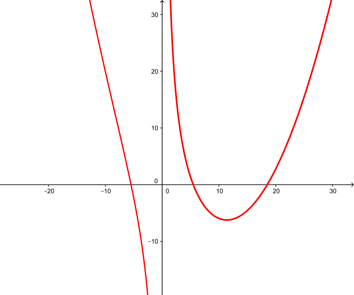
Figure 6. A Cartesian parabola
For constants \(n, a,\) and \(b,\) start with a parabola \(y=\frac{x^{2}}{n}\) with vertex D (D is the point \((0,0)\) to begin with). Place point E exactly \(a\) units above point D (E is the point \((0,a)\) to begin with). Then place the point A at \((b,0)\) and draw a line through A and E. This line intersects the parabola at two points, C1 and C2. For example, in Figure 7 below, \(n=10,\) \(a=3,\) and \(b=15\) (to begin with).
The parabola now ‘slides’ up and down in such a way that point E always remains \(a\) units above point D. Point A stays fixed so the line AE changes slope as E moves. Each possible location for the vertex creates new points C1 and C2 where line AE intersects the parabola. The locus of all the points C1 and C2 forms the two branches of the Cartesian parabola.
Figure 7. Constructing the Cartesian parabola. Instructions: Move the vertex D of the parabola up and down to see how the branches are formed. Move the sliders to adjust \(a, b,\) and \(n.\)
The equation for the two-branched Cartesian parabola, which will be derived later in this article, is the rational equation \[y=\frac{x^{2}}{n}-\frac{bx}{n}-a+\frac{ab}{x}.\] Notice that if you combine the fractions, you get a numerator of degree 3 and a denominator of degree 1, so this rational function has a vertical asymptote at \(x=0\) as well as a parabolic asymptote. Because of these features, the curve is a favorite with Precalculus instructors.
What makes this curve ‘simple’ is that it is based only on a line and a parabola, as opposed to, say, a graph of a cubic polynomial.
Descartes’ Method for Constructing Roots of Polynomials with ‘Simple’ Curves - Sextic and Quintic Equations
Constructing the roots of sextic and quintic equations using a circle and a Cartesian parabola
At the end of his 'Geometry,' Descartes tackled an incredible problem: to somehow construct the roots to polynomial equations of degree 6. Aside from occurring in modern algebra classes, Descartes pointed out that solutions to sextic equations arise in the following geometry problems:
- certain 9-, 10-, 11-, 12-, and 13-line locus problems (Smith 25),
- finding four mean proportionals (Smith 236, 239),
- dividing an angle into five equal pieces (Smith 239), and
- inscribing a regular 11-gon or 13-gon in a circle (Smith 239).
Earlier in his 'Geometry,' Descartes explained that any polynomial equation can be converted to one that has all positive roots by replacing \(x\) by \(x\) minus a constant \(c\) larger than the absolute values of all of the polynomial's negative roots. This is because the roots of \(f(x-c)\) will each be greater than the roots of \(f(x)\) by the positive value \(c,\) making each of the roots of \(f(x-c)\) positive. Though Descartes did not explain exactly how to determine the size of this constant, he did give some guidance, writing (Smith 168):
This can be done even when the false [negative] roots are unknown, since approximate values can always be obtained for them and the roots can then be increased by a quantity as large as or larger than is required.
Descartes claimed further that, "When this is done, there will be no two consecutive \(+\) or \(-\) terms" (Smith 168), and that the coefficient of the third largest exponent could be made bigger than the square of half the coefficient of the second largest exponent (Smith 168, 220). (See Note on Descartes' 'Rule of Signs'.)
After these preliminaries, Descartes tackled the problem of constructing the roots to any sixth degree polynomial of the form \[x^{6}+px^{5}+qx^{4}+rx^{3}+sx^{2}+tx+u=0,\] where the coefficients \(p, r,\) and \(t\) are negative, the coefficients \(q,s,\) and \(u\) positive, and \(q>\left({\frac{p}{2}}\right)^2.\) Again, he claimed that sextic equations that do not meet these constraints can be transformed by a substitution of variables. He noted further that quintics could be solved by multiplying through by \(x\) and solving the resultant sextic (ignoring the solution \(x=0\)).
I will first describe Descartes’ solution process and analyze it afterwards.
The roots to the sextic equation of the form \[x^{6}+px^{5}+qx^{4}+rx^{3}+sx^{2}+tx+u=0\] can be constructed as follows:
Step 1. Construct the right branch of a Cartesian parabola with (positive) parameters \[n=\sqrt{q-\frac{t}{\sqrt{u}}-\frac{p^{2}}{4}},\quad{a=-\frac{2\sqrt{u}}{pn}},\quad{\rm{and}}\quad{b=-\frac{p}{2}}.\]
Figure 8. First step of Descartes' process for solving sextic equations. Instructions: Change the values of \(p, q, r, s, t,\) and \(u\) to see how the shape of the right branch of the Cartesian parabola changes. (The values shown for \(p,r,\) and \(t\) on the sliders are absolute values.) You may slide the vertex of the parabola up and down the \(y\)-axis, as well, to see how the line and parabola form the right branch of the Cartesian parabola. To hide the parabola and the line, uncheck the ‘hide/show sliding parabola’ checkbox.
Step 2. To find the real solutions to the sextic equation, place a point L at \((0,-a),\) so that L is \(a\) units below the origin B, and place a point H at \((0,k)\) where \(k=-\frac{t}{2n\sqrt{u}}-a.\) The length of line segment LH, then, is \(a+k.\) Extend a line segment horizontally from H into the first quadrant a distance \(h\) to point I, where \[h=-\frac{r}{2n^{2}}+\frac{\sqrt{u}}{n^{2}}+\frac{pt}{4n^{2}\sqrt{u}}.\] Construct a circle with LI as its diameter. Construct another circle with center L and radius \(\sqrt{\frac{s-p\sqrt{u}}{n^{2}}}\) and call one (or both) of the intersection points of the two circles P.
Figure 9. Second step of Descartes' process for solving sextic equations. Instructions: Change the values of the coefficients \(p, q, r, s, t,\) and \(u\) to see how the Cartesian parabola, the circles, and the triangle change.
Step 3. Finally, construct a circle with center I which passes through point P. Then the \(x\)-coordinates of the intersections of that circle with the Cartesian parabola are the roots of the original equation.
Figure 10. Third step of Descartes' process for solving sextic equations. Instructions: Change the values of \(p, q, r, s, t,\) and \(u\) to see how the intersections with the circle change to give the real solutions to the sextic equation. By adjusting the values of the coefficients, you can obtain examples of degree 6 polynomials having four, two, and no positive real roots, along with, respectively, two, four, and six imaginary roots. This leaves one case, that of six positive real roots.
Here is the actual diagram from the 'Geometria,' in which Descartes' axes are oriented in the opposite direction of how we orient them today. Point B is the origin, point D is the vertex of the sliding parabola, point A is the fixed point of the intersecting line segment, point C is a point on the Cartesian parabola, and point I is the center of the circle.

Figure 11. Descartes' method for finding solutions for degree 6 polynomials. The diagram above appears in Frans van Schooten's translation of Descartes' French ‘La Géométrie’ into the Latin 'Geometria.' Van Schooten's first edition appeared in 1649; this image is from his 1659 second edition, available via Google Books. The original diagram appeared in Descartes' 1637 ‘La Géométrie’ on page 404 of his longer Discours de la Methode and on page 222 of Smith's and Latham's facsimile (and English translation) of ‘La Géométrie.’
Descartes merely stated his process and, for his ‘proof,’ showed that by starting with \(b, n, a, h, k,\) and radius IP in terms of \(p, q, r, s, t,\) and \(u,\) the intersections would correspond to roots of the sextic equation \[x^{6}+px^{5}+qx^{4}+rx^{3}+sx^{2}+tx+u=0.\] It will be shown later in this article how to derive \(b, n, a, h, k,\) and radius IP from the coefficients \(p, q, r, s, t,\) and \(u\) of the polynomial. First, we'll consider an example of a sixth degree polynomial with six positive real roots.
Note on Descartes' 'Rule of Signs'
If all of the roots of a polynomial are real, Descartes' own "rule of signs" guarantees that the coefficients of the polynomial must alternate between \(+\) and \(-\) in order for all of its roots to be positive. In this case, if the polynomial does have some negative roots, the signs will not alternate throughout, but if the function \(f(x-c)\) for big enough \(c\) is created then the signs of the coefficients of the new polynomial will alternate and its roots will all be positive.
Descartes stated his famous "rule of signs" a few pages before the discussion cited above (Smith 160):
An equation can have as many true [positive] roots as it contains changes of sign, from \(+\) to \(-\) or from \(-\) to \(+\); and as many false roots as the number of times two \(+\) signs or two \(-\) signs are found in succession.
This statement allows for the possibility of complex roots, and Descartes applied his strategy described above for making all negative roots positive to polynomials with both real and complex roots. One way to be certain all real roots are positive is to make sure the signs of the coefficients of the polynomial alternate between \(+\) and \(-\) throughout. However, a sixth degree polynomial, for instance, can have 0, 2, 4, or 6 complex roots (since complex roots occur in pairs) and 6, 4, 2, or 0 positive real roots, respectively. In all four cases, all of the real roots are positive, but, according to Descartes' "rule of signs," only the case of six positive real roots requires six sign changes. We consider the special case of a sixth degree polynomial with six positive real roots on the next webpage.
Descartes’ Method for Constructing Roots of Polynomials with ‘Simple’ Curves - Sixth Degree Equations with Six Real Positive Roots
About his process for finding roots of sixth degree polynomials, Descartes wrote (Smith 224):
This rule never fails nor does it admit of any exceptions.
Yet his one example is a specific type with just four real roots that seems somewhat contrived. Just as a circle can intersect a parabola in four points, it would seem logical that it should only be able to intersect the right branch of Descartes' ‘parabola of the second order’ in four points as well. But what if the polynomial has six real roots?
For example, the equation \[x^{6}-6x^{5}-15x^{4}+88x^{3}+64x^{2}-168x+36=0\] has two negative roots and four positive roots. Descartes would have us replace \(x\) with \(x-4\) to get the equation \[x^{6}-30x^{5}+345x^{4}-1912x^{3}+5248x^{2}-6440x+2500=0\] and then create the circle and right branch of the Cartesian parabola, confident that they will intersect six times at the proper places. Though a standard parabola can only intersect a circle in at most four places, the Cartesian parabola can, indeed, intersect a circle at six points.
Figure 12. Sextic equation with six real roots. Change the values of the roots to see how the circle and Cartesian parabola vary.
On the second to last page of 'The Geometry,' Descartes admitted (Smith 239):
[I]n many of these problems it may happen that the circle cuts the parabola of the second class so obliquely that it is hard to determine the exact point of intersection. In such cases this construction is not of practical value. The difficulty could easily be overcome by forming other rules analogous to these, which might be done in a thousand different ways.
Rather than hint at a thousand ways to resolve this issue, there was a simple one that Descartes seems to have chosen not to reveal. He could have relaxed his restriction on the roots having to all be positive and also utilized the left branch of the Cartesian parabola, which he described and used in Book II (Smith 87) in his solution to another problem known as the ‘five line locus problem.’
In the applet above, slide the offset all the way to the left so that each of the roots is reduced by \(4.\) The new circle will intersect the right branch of the Cartesian parabola in four places and the left branch of the Cartesian parabola in two places.
The original equation was \[x^{6}-6x^{5}-15x^{4}+88x^{3}+64x^{2}-168x+36=0.\]
Using Descartes’ formulas, we get values \(b=3, n=2, a=1, h=1,\) and \(k=6,\) and radius \({\rm{IP}}=5.\) Also, point \((h,k)\) is the center of the circle, and the equation of the Cartesian parabola is \[y=\frac{x^{2}}{2}-\frac{3x}{2}-1+\frac{3}{x}.\] When the offset is set to –4 in Figure 12, above, the intersections of the circle and two-branched Cartesian parabola give as the six roots of the original equation, \(x\approx -3.30968,\) \(x\approx -1.85769,\) \(x\approx 0.244316,\) \(x=1,\) \(x\approx 4.15473,\) and \(x\approx 5.76832.\)
Descartes’ Method for Constructing Roots of Polynomials with ‘Simple’ Curves - Derivation of Descartes' Method: Cartesian Parabola
Descartes did not explain his derivations, writing (Smith 192):
I have also omitted here the demonstration of most of my statements, because they seem to me so easy that if you take the trouble to examine them systematically the demonstrations will present themselves to you and it will be of much more value to you to learn them in that way than by reading them.
And later, as the final sentence of his book, he wrote (Smith 240):
I hope that posterity will judge me kindly, not only as to the things which I have explained, but also as to those which I have intentionally omitted so as to leave to others the pleasure of discovery.
Descartes did not explain how he derived the complex rules that convert the coefficients \(p, q, r, s, t,\) and \(u\) of the given sextic equation into the six parameters \(n, a, b, h, k,\) and \(d\) for defining the Cartesian parabola and the circle. All he did was verify that these complex rules are correct by algebraically finding the intersection of the Cartesian parabola and the circle and showing that it leads to the proper sextic equation.
Before taking on the challenge of rediscovering Descartes’ daunting construction, I searched for previously published analyses of his work. In the College Mathematics Journal (18, 1987), I found a nice derivation of the formula for the Cartesian parabola in an article about Isaac Newton by V. Frederick Rickey. Newton dubbed this curve the ‘trident’ as it resembles the pitchfork wielded by the sea god.
Deriving the formula for the Cartesian parabola
In Figure 13, below, point B is the origin, lengths \({\rm{BA}}=b\) and \({\rm{DE}}=a\) are fixed, and variable lengths \({\rm{CG}}=y\) and \({\rm{CF}}=x\) are coordinates of the point C on both the Cartesian parabola and the ordinary parabola. Therefore, the equation of the (ordinary) parabola is \[y=\frac{x^{2}}{n}+{\rm{BD}}\] (with BD changing as the parabola slides up and down) and \({\rm{GA}}=b-x.\) By similar triangles, \(\frac{b-x}{y}=\frac{x}{\rm{FE}},\) so \({\rm{FE}}=\frac{xy}{b-x}.\) Also, when D coincides with B, FD is the \(y\)-value for each point on the parabola, so \[{\rm{FD}}=\frac{{\rm{FC}}^{2}}{n}=\frac{x^{2}}{n}.\]
Figure 13. Deriving the equation for the Cartesian parabola. Instructions: Move the vertex of the parabola up and down. The parameters \(n, a,\) and \(b\) can be adjusted with the sliders.
But \[{\rm{FD}}={\rm{DE}}-{\rm{FE}}=a-{\rm{FE}}=a-\frac{xy}{b-x}.\] Equating two expressions for FD, we can say \[\frac{x^{2}}{n}=a-\frac{xy}{b-x}=\frac{ab-ax-xy}{b-x}.\] Clear the denominators to get \[bx^2-x^{3}=nab-nax-nxy.\] Now isolate \(nxy\): \[nxy=nab-nax-bx^{2}+x^{3}\] and solve for \(y\) to get: \[y=\frac{x^{2}}{n}-\frac{bx}{n}-a+\frac{ab}{x}\] as the equation of the Cartesian parabola (Rickey 372).
From the equation of the Cartesian parabola, and knowing already what Descartes’ results were, I next set out to re-derive Descartes’ parameters for his construction – that is, starting with the coefficients of a sextic equation, to come up with the center and radius of the circle and also the two parameters that define the Cartesian parabola so that the \(x\)-intercepts of the intersections of the circle and Cartesian parabola would equal the real roots of the sextic equation.
Descartes’ Method for Constructing Roots of Polynomials with ‘Simple’ Curves - Derivation of Descartes' Method: Parameters
Finding relationships between parameters using a system of six equations and six unknowns
From the equation of the Cartesian parabola, \(y=\frac{x^{2}}{n}-\frac{bx}{n}-a+\frac{ab}{x},\) and knowing already what Descartes’ results were, I tackled the challenge of re-deriving Descartes’ parameters for his construction – starting with the coefficients of a sextic equation to come up with the center and radius of the circle and also of the two parameters that define the Cartesian parabola so that the \(x\)-intercepts of the intersections would equal the real roots of the sextic equation.
The Cartesian parabola has three parameters, \(n\) (the coefficient of \(y\) in the original sliding parabola), \(b\) (the fixed \(x\)-intercept of the line that intercepts the sliding parabola), and \(a\) (the \(y\)-intercept of the line, which is always the same distance above the vertex of the sliding parabola). The circle has three parameters, \(h\) (the \(x\)-coordinate of the center of the circle), \(k\) (the \(y\)-coordinate of the center of the circle), and the radius of the circle, \(d.\) The goal is to relate these to the six coefficients of the sextic equation \(p, q, r, s, t,\) and \(u.\)
To find these relations, substitute \(y=\frac{x^{2}}{n}-\frac{bx}{n}-a+\frac{ab}{x}\) into the equation \((x-h)^{2}+(y-k)^{2}=d^{2}.\) Combine like terms and multiply through by \(x^{2}n^{2}\) to get the equation:
\[x^{6}-2bx^{5}+(n^{2}-2kn+b^{2}-2an)x^{4}+(-2hn^{2}+2bkn+4abn)x^{3}\]
\[+(-n^{2}d^{2}+k^{2}n^{2}+h^{2}n^{2}+2akn^{2}-2ab^{2}n+a^{2}n^{2})x^{2}\]
\[+(-2abkn^{2}-2a^{2}bn^{2})x+a^{2}b^{2}n^{2}=0.\]
Equate coefficients with those of \[x^{6}+px^{5}+qx^{4}+rx^{3}+sx^{2}+tx+u=0\] to get the system of equations:
- \(p=-2b\)
- \(q=n^{2}-2kn+b^{2}-2an\)
- \(r=-2hn^{2}+2bkn+4abn\)
- \(s=-n^{2}d^{2}+k^{2}n^{2}+h^{2}n^{2}+2akn^{2}-2ab^{2}n+a^{2}n^{2}\)
- \(t=-2abkn^{2}-2a^{2}bn^{2}\)
- \(u=a^{2}b^{2}n^{2}\)
From these six equations in six unknowns, the goal is to somehow solve for \(a, b, d, n, h,\) and \(k\) in terms of \(p, q, r, s, t,\) and \(u.\)
Solving for b
Divide both sides of equation (1) by \(-2\) to get \(b=-\frac{p}{2}.\)
Solving for n
Equation (2) can be rearranged to read \(n^{2}=q+2kn+2an-b^{2}\) or \(n={\sqrt{q+2kn+2an-b^2}}.\) From equation (6), \({\sqrt{u}}=abn.\) Substituting \(abn = {\sqrt{u}}\) into equation (5) yields \({\frac{t}{\sqrt{u}}}=-2kn-2an\) and \(-{\frac{t}{\sqrt{u}}}=2kn+2an,\) which are equivalent to the second and third term under the radical in the rearrangement of equation (2). Also, since \(b=-\frac{p}{2}\) so that \(b^2={\frac{p^2}{4}},\) we have \[n=\sqrt{q-\frac{t}{\sqrt{u}}-\frac{p^{2}}{4}}.\]
Solving for a
That \(a=\frac{2abn}{2bn},\) \(abn=\sqrt{u},\) and \(2b=-p\) yields \(a=\frac{2\sqrt{u}}{-pn},\) or \(a=-\frac{2\sqrt{u}}{pn}.\)
Solving for k
Solve for \(k\) in equation (5), \(t=-2abkn^{2}-2a^{2}bn^{2},\) to get \(k=\frac{t}{-2n(abn)}-a.\) Substitute \(abn=\sqrt{u}\) and \(a=-\frac{2\sqrt{u}}{pn}\) into this equation to obtain \(k =-\frac{t}{2n\sqrt{u}}+\frac{2\sqrt{u}}{pn}.\)
Solving for h
Solve for \(h\) in equation (3), \(r=-2hn^{2}+2bkn+4abn,\) to get \(h=-\frac{r}{2n^{2}}+\frac{2abn}{n^{2}}+\frac{2bkn}{2n^{2}}.\) Substitute \(abn=\sqrt{u}\) and \(2b=-p\) into this equation to obtain \(h=-\frac{r}{2n^{2}}+\frac{2\sqrt{u}}{n^{2}}-\frac{pkn}{2n^{2}}.\) This last equation can be rewritten as follows:
\(h=-\frac{r}{2n^{2}}+\frac{\sqrt{u}}{n^{2}}+\frac{\sqrt{u}}{n^{2}}-\frac{2pkn\sqrt{u}}{4n^{2}\sqrt{u}} = -\frac{r}{2n^{2}}+\frac{\sqrt{u}}{n^{2}}+\frac{4u-2pkn\sqrt{u}}{4n^{2}\sqrt{u}}.\)
Substitute \(\sqrt{u}=abn\) and \(p=-2b\) back into the numerator of the third term to get:
\(h=-\frac{r}{2n^{2}}+\frac{\sqrt{u}}{n^{2}}+\frac{4a^{2}b^{2}n^{2}-2(-2b)knabn}{4n^{2}\sqrt{u}}=-\frac{r}{2n^{2}}+\frac{\sqrt{u}}{n^{2}}+\frac{-2b(-2a^{2}bn^{2}-2abkn^{2})}{4n^{2}\sqrt{u}}.\)
Finally, substitution of \(-2b=p\) and equation (5), \(-2abkn^{2}-2a^{2}bn^{2}=t,\) into the third term yields \[h=-\frac{r}{2n^{2}}+\frac{\sqrt{u}}{n^{2}}+\frac{pt}{4n^{2}\sqrt{u}}.\]
Solving for d
Solve for \(d^2\) in equation (4), \(s=-n^{2}d^{2}+k^{2}n^{2}+h^{2}n^{2}+2akn^{2}-2ab^{2}n+a^{2}n^{2},\) to get:
\(d^{2}=-\frac{s}{n^2}+k^{2}+h^{2}+2ak-\frac{2ab^{2}}{n}+a^{2}=(a+k)^{2}+h^{2}-\frac{s+2a{b^2}n}{n^{2}}.\)
Substitute \(abn=\sqrt{u}\) and \(2b=-p\) into the last term to obtain \(d^{2}=(a+k)^{2}+h^{2}-\frac{s-p\sqrt{u}}{n^{2}},\) or
\[d=\sqrt{(a+k)^{2}+h^{2}-\frac{s-p\sqrt{u}}{n^{2}}}.\]
At this point, Descartes had all six parameters \(a, b, n, h, k,\) and \(d\) expressed in terms of the coefficients of the sextic equation \(p, q, r, s, t,\) and \(u.\) Here, \(a, b,\) and \(n\) define the Cartesian parabola and \((h,k)\) and \(d\) define the center and radius of the circle.
The final piece that bears explaining is how, after Descartes created the Cartesian parabola and the center of the circle at point \((h,k),\) he created the circle itself.
Descartes’ Method for Constructing Roots of Polynomials with ‘Simple’ Curves - Derivation of Descartes' Method: Circle Construction
Constructing the circle
At this point, Descartes had parameters \(a, b,\) and \(n\) defining the Cartesian parabola and \(h, k,\) and \(d\) defining the center and radius of the circle. The final piece that bears explaining is that after Descartes created the Cartesian parabola and the center of the circle at point \((h,k)\) (point I on the diagram), he did something cryptic to create the circle itself.
Figure 14. Cartesian parabola and point I. Instructions: Change the values of \(p, q, r, s, t,\) and \(u\) to change the Cartesian parabola and the location of point I.
Rather than just say to construct a circle with a radius of length \(d=\sqrt{(a+k)^{2}+h^{2}-\frac{s-p\sqrt{u}}{n^{2}}},\) Descartes instead created two circles, one with diameter IL where B is the origin and BL is of length \(a,\) and another circle with center L and radius \(\sqrt{\frac{s-p\sqrt{u}}{n^{2}}}.\) The intersection, P, of these two circles, he claimed, would be a point (or points) on the circle with center I and radius \[d=\sqrt{(a+k)^{2}+h^{2}-\frac{s-p\sqrt{u}}{n^{2}}}.\]
Figure 15. Two circles are used to create the main (green) circle. Instructions: Adjust the coefficients \(p, q, r, s, t,\) and \(u\) to see how the Cartesian parabola, three circles, and triangle change.
To see why this works, look at triangles HIL and PIL, which are both right triangles with diameter LI as their hypotenuses.
Figure 16. Construction of line segment IP. Instructions: Drag points H, I, L, and P to see that IP will have length \(\sqrt{{\rm{LH}}^2+{\rm{HI}}^2-{\rm{PL}}^2}.\)
To give IP the length \[d=\sqrt{(a+k)^{2}+h^{2}-\frac{s-p\sqrt{u}}{n^{2}}},\] Descartes used the fact that, in a circle with diameter LI and points H and P on the circumference, two right triangles LPI and LHI sharing hypotenuse LI are formed. Since \[{\rm{LI}}^{2}={\rm{PL}}^{2}+{\rm{IP}}^{2}={\rm{LH}}^{2}+{\rm{HI}}^{2},\] we have \[{\rm{IP}}=\sqrt{{\rm{LH}}^2+{\rm{HI}}^2-{\rm{PL}}^2}.\] By making \({\rm{LH}}=a+k,\) \({\rm{HI}}=h,\) and \({\rm{PL}}=\sqrt{\frac{s-p\sqrt{u}}{n^{2}}},\) IP will then have the required length \[d=\sqrt{(a+k)^{2}+h^{2}-\frac{s-p\sqrt{u}}{n^{2}}}.\]
Descartes’ Method for Constructing Roots of Polynomials with ‘Simple’ Curves - Conclusion, References, and About the Author
Conclusion
As noted at the start of my derivation of Descartes' method for solving sextic equations, Descartes did not explain his derivations, writing in his 'Geometry' (Smith 192):
I have also omitted here the demonstration of most of my statements, because they seem to me so easy that if you take the trouble to examine them systematically the demonstrations will present themselves to you and it will be of much more value to you to learn them in that way than by reading them.
And later, as the final sentence of his book, he wrote (Smith 240):
I hope that posterity will judge me kindly, not only as to the things which I have explained, but also as to those which I have intentionally omitted so as to leave to others the pleasure of discovery.
Attempting to reconstruct Descartes’ thought process was not as ‘pleasurable’ for me as he might have intended, but it was certainly satisfying.
References
Boyer, Carl B. History of Analytic Geometry. Mineola, NY: Dover Publications, 2004. Originally published in Scripta Mathematica Studies series (New York), 1956. Print.
Descartes, René. 'La Géométrie,' in The Geometry of René Descartes (David Eugene Smith and Marcia L. Latham, translators). New York, NY: Dover Publications, 1996, 1954. Originally published by Open Court Publishing Co., 1925. Print.
Katz, Victor and Karen Parshall. Taming the Unknown: A History of Algebra from Antiquity to the Early Twentieth Century. Princeton University Press, 2014. Print.
Knorr, Wilbur Richard. The Ancient Tradition of Geometric Problems. New York: Dover, 1993. Originally published by Birkhäuser (Boston), 1986. Print.
Rickey, V. Frederick, ‘Isaac Newton: Man, Myth, and Mathematics,’ College Mathematics Journal 18 (1987), pp. 362-389.
Smith, David Eugene and Marcia L. Latham (translators). The Geometry of René Descartes. New York, NY: Dover Publications, 1996, 1954. Originally published by Open Court Publishing Co., 1925. Print. Same work as in entry for "Descartes, René," above. Since all references to this work in the present article are to the English translation, citations are to Smith rather than to Descartes.
Additional Reading
For a list of easy-to-access publications of Descartes' 'Geometry' in English, French, and Latin, see the Convergence article, "The Geometry of René Descartes."
For more about the history of solving quadratic equations, see the Convergence article, "Geometric Algebra in the Classroom" (reprint of "Geometric Approaches to Quadratic Equations from Other Times and Places").
To see how Omar Khayyam solved a cubic equation, see the Convergence article, "A GeoGebra Rendition of One of Omar Khayyam's Solutions for a Cubic Equation."
About the Author
Gary Rubinstein is a mathematics teacher at Stuyvesant High School in the Borough of Manhattan, New York, New York. One of nine public high schools in New York City with specialized and accelerated curricula, Stuyvesant is a college preparatory high school specializing in STEM subjects. Rubinstein was awarded Math for America Master Teacher Fellowships in 2006, 2010, and 2014.