A Series of Mini-projects from TRIUMPHS: TRansforming Instruction in Undergraduate Mathematics via Primary Historical Sources
Regular readers of Convergence are unlikely to need to be convinced of the value of studying primary sources in order to understand the development of mathematics. Essentially all good scholarship in mathematics is necessarily based on primary sources. But, as many have come to recognize, primary source materials are also valuable in learning the subject. Thanks in part to the work of David Pengelley [11], Jerry Lodder [10], Janet Barnett [3], and others [1,2,5,6,12], ideas about the incorporation of primary sources in the teaching of university mathematics have become increasingly well-known over the last few decades. Dozens of mathematics faculty have given talks recently at national meetings about this pedagogical innovation, and several articles in Convergence have described details of such an approach [7,8,9,13,14], and even provided collections of classroom-ready student projects based on primary sources [4].
An outside observer, seeing this significant increase in the attention paid to the role of primary sources in teaching, may think that the movement to promote this method of teaching has been successful, and that these techniques are now widely used.
Some of us, however, share the view that the techniques are not nearly mainstream enough. That faculty with an interest in primary sources can use them in their teaching is well and good, but we are convinced that there are so many benefits derived from their use that we would like to see them available to all instructors of university mathematics.


Students work on a Primary Source Project under the supervision of Janet Heine Barnett at a
TRIUMPHS Site Tester Workshop, held at the University of Colorado, Denver, during September 2016.
Five years ago, at a workshop for the NSF-funded project Learning Discrete Mathematics and Computer Science via Primary Historical Sources in Las Cruces, New Mexico, a group of us started planning a large project: a national, funded, extended effort to build on the successful work done over the previous decades to promote this work of teaching with primary sources and help to make it more common. We would do this by continuing to prepare ready-to-use curriculum materials in the form of classroom projects based on primary source materials through which students could learn a wide variety of standard topics in university mathematics classes. If more such projects were available, we reasoned, they might significantly reduce the perceived difficulty some instructors may have in using original sources for the first time, especially if this broader collection of projects included a variety of shorter projects. Furthermore, if we combined the work of disseminating these projects with a careful research plan, we might learn something important about the benefits or barriers of using such an approach.
In 2015, our group, which had by this time expanded to a team of seven, secured a Collaborative Research grant from the National Science Foundation of about $1.5 million over five years to run this grand experiment on a large scale. We have been working actively since then first to write and edit these “Primary Source Projects”, or PSPs, then to test them in classrooms – either our own or in those of colleagues at other institutions.
The grant effort, TRansforming Instruction in Undergraduate Mathematics via Primary Historical Sources (or TRIUMPHS), is well underway, and we encourage readers to find out more about its current status at the TRIUMPHS website. In addition to administrative notices governing the work of the grant, we maintain there an updated set of PSPs, available for perusal and download.
We’d especially like to call attention to a new set of "mini-PSPs" which takes our work in an exciting new direction. These shorter Primary Source Projects are designed to be completed within one or two class periods, and to give instructors already familiar with primary sources more flexibility in their use. We plan to publish a series of these mini-PSPs in Convergence over the next few years - beginning with the mini-PSP The Derivatives of the Sine and Cosine Functions - and we invite the mathematical community to read and use them.
If readers do decide to use projects in their classes, of course, we would love to know about it – contact the project’s author or any member of the TRIUMPHS team in advance, and we’ll be happy to talk with you. And have fun exploring them!

Subset of TRIUMPHS PIs and Advisory Board Members: David Pengelley, Diana White,
Danny Otero, Dominic Klyve, Janet Heine Barnett, Kathy Clark, Nick Scoville.
Acknowledgments
This material is based upon work supported in part by the National Science Foundation under Grants No. 1523494, 1523561, 1523747, 1523753, 1523898, 1524065, and 1524098. Any opinions, findings, and conclusions or recommendations expressed in this material are those of the author(s) and do not necessarily reflect the views of the National Science Foundation.
References
- J. Barnett, G. Bezhanishvili, J. Lodder, and D. Pengelley, Teaching Discrete Mathematics Entirely From Primary Historical Sources, PRIMUS: Problems, Resources and Issues in Mathematics Undergraduate Studies, 26 (2016) no. 7, 657-675, DOI 10.1080/10511970.2015.1128502.
- J. Barnett, J. Lodder, and D. Pengelley, Teaching and Learning Mathematics From Primary Historical Sources, PRIMUS: Problems, Resources and Issues in Mathematics Undergraduate Studies, 26 (2016) no. 1, 1 - 18, DOI 10.1080/10511970.2015.1054010.
- J. Barnett, Learning mathematics via primary historical sources: Straight from the source’s mouth, PRIMUS: Problems, Resources and Issues in Mathematics Undergraduate Studies: Special Issue on the Use of History of Mathematics to Enhance Undergraduate Mathematics Instruction, 24 (2014), no. 8, 722–736, DOI:10.1080/10511970.2014.899532.
- J. Barnett, G. Bezhanishvili, H. Leung, J. Lodder, D. Pengelley, I. Pivkina, D. Ranjan, and M. Zack, Primary Historical Sources in the Classroom: Discrete Mathematics and Computer Science, Loci: Convergence (July 2013), DOI 10.4169/loci003984.
- J. Barnett, H. Leung, J. Lodder, D. Pengelley, and D. Ranjan, Designing Student Projects for Teaching and Learning Discrete Mathematics and Computer Science via Primary Historical Sources, in Recent Developments on Introducing a Historical Dimension in Mathematics Education (V. Katz and C. Tzanakis, eds.), Mathematical Association of America, Washington DC, 2011, 187–198.
- J. Barnett, J. Lodder, and D. Pengelley, The pedagogy of primary historical sources in mathematics: Classroom practice meets theoretical frameworks, Science & Education: Special Issue on the Philosophy and History of Mathematics in Mathematics Education 23 (2014), no. 1, 7–27.
- K. M. Clark, 'In these numbers we use no fractions': A Classroom Module on Stevin's Decimal Fractions - Overview and Introduction, Loci: Convergence (January 2011), DOI:10.4169/loci003333.
- A. Dematte, Introducing the History of Mathematics: An Italian Experience Using Original Documents, Loci: Convergence (February 2010), DOI:10.4169/loci002856
- D. Klyve, L. Stemkowski, and E. Tou, Teaching and Research with Original Sources from the Euler Archive, Loci: Convergence (April 2011), DOI 10.4169/loci003672.
- J. Lodder, Networks and spanning trees: the juxtaposition of Prüfer and Borůvka. PRIMUS: Problems, Resources and Issues in Mathematics Undergraduate Studies: Special Issue on the Use of History of Mathematics to Enhance Undergraduate Mathematics Instruction, 26 (2016) 24 (2014), no. 8, 737 -751, DOI: 10.1080/10511970.2014.896835.
- D. Pengelley, Teaching with primary historical sources: Should it go mainstream? Can it?, in Recent Developments on Introducing a Historical Dimension in Mathematics Education (V. Katz and C. Tzanakis, eds.), Mathematical Association of America, Washington DC, 2011, 1–8.
- D. Ruch, Creating a Project on Difference Equations with Primary Sources: Challenges and Opportunities, PRIMUS: Problems, Resources and Issues in Mathematics Undergraduate Studies: Special Issue on the Use of History of Mathematics to Enhance Undergraduate Mathematics Instruction, 24 (2014), no. 8, 764–773, DOI: 10.1080/10511970.2014.896836.
- N. Scoville, Georg Cantor at the Dawn of Point-Set Topology, Loci: Convergence (March 2012), DOI: 10.4169/loci003861.
- L. Stemkoski, Investigating Euler's Polyhedral Formula Using Original Sources - Original Sources: Who, What, Where, How, Convergence (April 2010), DOI:10.4169/loci003297.
Babylonian Numeration: A Mini-Primary Source Project for Pre-service Teachers and Other Students
When teaching any new topic, instructors face a dizzying number of choices about how to do so. Among these is: how much scaffolding should be provided? At the risk of oversimplifying, answers to this question lie along a spectrum. At one end, some traditional teaching methodologies give students all of the theorems, methods, or rules relating to the topic at hand. At the other extreme, some “Discovery Learning” methodologies provide students with almost no information, instead offering an extended series of leading questions that encourage them to build their own knowledge. The purpose of this article is not to revisit the complex question of the benefits or drawbacks of these methods, but to provide an example at one end of these extremes that makes use of the history of mathematics: the mini-Primary Source Project Babylonian Numeration.
Exploring the Babylonian numeration system in general presents a marvelous opportunity, for students who are not familiar with it, to challenge basic assumptions about numerical representation. While this system shares certain features with the more familiar Hindu-Arabic base-10 numeration system (e.g., the use of position to convey the value of each symbol), it differs significantly in other respects (e.g., base 60, use of only two distinct symbols) that cause the two systems to look quite dissimilar.
Many books that teach numeration using Akkadian cuneiform take a more traditional approach in laying out the rules for base-60 numeration; some even use Hindu-Arabic numerals to represent the values within each “place value” (the Hindu-Arabic numeral 72, for example, might be written as “60 12” in the Babylonian system). The Primary Source Project Babylonian Numeration, at the other extreme, provides students no clue as to how the system works, no familiar numerals to hold on to, and not even a clean depiction of the numerals themselves. Thrown in at the deep end, as it were, students must find their own way to land.
The project itself is quite straightforward: students are given a representation of a tablet and asked to work out for themselves both the structure of the Babylonian system and the mathematics depicted on the tablet. Instructors are left to decide the actual visual format of the tablet that they wish to present to students, which could take several forms. Consider the following two representations of a Babylonian tablet:


(Readers are invited, at this point, to work out for themselves the mathematics depicted.)
The image on the left is, of course, a photograph of the front side of the tablet on which the PSP is based: Tablet HS 224 in the Hilprecht Collection at the University of Jena (photographer C. Proust, Cuneiform Digital Library Initiative). The image on the right is an attempt to faithfully represent the tablet as it has been preserved: Image 26 on Plate 16 in [Hilprecht 1906]. The two images contain similar information; the one on the right, however, is easier to read.
We could, of course, go a step further and clean up the symbols for the student, as in the following:

There may be good reasons to do this, but in practice the author has found that letting students grapple with the missing information only increases their level of productive struggle, and increases their pride when they work out the mathematics involved. Indeed, the students, who usually succeed in determining what’s going on—possibly with a few hints—are generally thrilled with their accomplishment.
The complete project Babylonian Numeration (pdf) is ready for student use, and the LaTeX source code is available from the author by request. Instructors are welcome to change the image and to make different choices regarding the presentation of the tablet if they wish. If they do, of course, the author would love to hear the results of their experiment. A set of instructor notes that explain the purpose of the project and guide the instructor through its goals is appended at the end of the student project.
This project is the seventeenth in A Series of Mini-projects from TRIUMPHS: TRansforming Instruction in Undergraduate Mathematics via Primary Historical Sources appearing in Convergence, for use in courses ranging from first-year calculus to analysis, number theory to topology, and more. Links to other mini-PSPs in the series appear below. The full TRIUMPHS collection also offers dozens of other mini-PSPs and a similar number of more extensive full-length PSPs.
Acknowledgments
The author is grateful to Dr. Christine Proust (Centre National de la Recherche Scientifique and Paris Diderot University), for providing information about and permission to use her photograph of the tablet in this article and the mini-PSP itself. The development of the student project Babylonian Numeration has been partially supported by the TRansforming Instruction in Undergraduate Mathematics via Primary Historical Sources (TRIUMPHS) project with funding from the National Science Foundation’s Improving Undergraduate STEM Education Program under Grants No. 1523494, 1523561, 1523747, 1523753, 1523898, 1524065, and 1524098. Any opinions, findings, and conclusions or recommendations expressed in this project are those of the author and do not necessarily reflect the views of the National Science Foundation.
References
Hilprecht, Hermann Vollrat. 1906. The Babylonian Expedition of the University of Pennsylvania. Series A: Cuneiform Texts, Volume 20. Philadelphia: University of Pennsylvania Press.
Beyond Riemann Sums: Fermat's Method of Integration – A Mini-Primary Source Project for First-Year Calculus Students
For those of us who have studied (or taught) calculus for years, the idea of approximating the area under a curve with Riemann sums may seem so self-evident as to not merit much consideration. What could be simpler than starting with an interval, splitting it into subintervals of equal size, and finding an approximation to the area under the curve over each of these intervals? On the other hand, might there exist other methods that are historically-grounded and ripe for student exploration? The rhetorical nature of the previous questions being obvious, the reader will not be surprised to know that the answer is “yes—and this article introduces a mini-Primary Source Project (mini-PSP), Beyond Riemann Sums: Fermat's Method of Integration, designed to introduce students in a first course on integration to one such method.”
Of course, if a curve has properties that make it behave differently over different areas of its domain, we might start to guess that there could be a more clever method to estimate this area. Indeed, many areas of mathematical modeling, numerical analysis, or statistics rely on the idea that approximating methods can “zoom in” to areas where a lot of change happens, but give coarser approximations when the underlying curve (or model) is more static. Perhaps, a historian might speculate, after Riemann gave us regular intervals, another mathematician proposed a method that bases the size of the approximating rectangles on the absolute value of the derivative of the function to be approximated, as shown in the following figure.
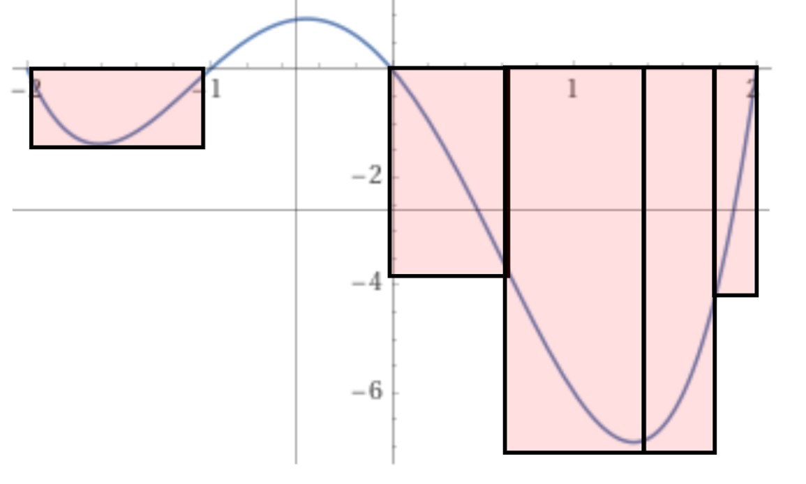
Finding a lower bound on \(\int_{-2}^2 f(x) dx\) using rectangles of variable width.
Image created by the author.
However, in one of those twists that seems to be common in the history of calculus, the first proposal to find the area under a curve using rectangles of different sizes came not after Riemann, but before him. Indeed, before Euler, and before even Newton and Leibniz, Pierre de Fermat (1601–1665) proposed a method to find the “quadrature”—what we might now call the area under the curve—of the generalized hyperbola \(1/x^n\).
This mini-PSP walks students through Fermat’s method by using excerpts from his “Treatise on Quadratures”1 [Fermat 1679]. There are some challenges to reading Fermat’s work. Since it predates both the notion of the integral and function notation, Fermat worked only geometrically. However, what we lose from convenient notation we may gain from the understanding that comes through geometric reasoning. The project begins with Fermat’s discussion of the convergence of a geometric series, and then it introduces the method he used to find the area under a hyperbola using rectangles of different widths. Students are encouraged to use geometric thinking to find the area of these rectangles, and from these areas to deduce a conclusion about the area under the curve. In addition to seeing a nice example of mathematical invention as they explore Fermat’s clever trick, it is hoped that students will benefit from seeing all the main ideas of Riemann integration in this new, somewhat alien setting.

Fermat’s rectangles of different widths for estimating the area under a hyperbolic curve, from [Fermat 1679, p. 45].
The complete project Beyond Riemann Sums: Fermat's Method of Integration (pdf) is ready for student use and the LaTeX source code is available from the author by request. Instructor notes are provided to explain the purpose of the project and guide the instructor through implementation of the project.
This project is the twenty-eighth in A Series of Mini-projects from TRIUMPHS: TRansforming Instruction in Undergraduate Mathematics via Primary Historical Sources appearing in Convergence, for use in courses ranging from first-year calculus to analysis, number theory to topology, and more. Links to other mini-PSPs in the series, including 14 additional projects for use in introductory calculus courses, appear below. The full TRIUMPHS collection also offers two other mini-PSPs and six more extensive “full-length” PSPs for use in teaching calculus.
Recommendations for Further Reading
Without a doubt, the most thorough study of Fermat’s work is Michael Sean Mahoney’s The Mathematical Career of Pierre de Fermat (1601–1665) [Mahoney 1994]. Mahoney’s discussion of Fermat’s “Treatise on Quadrature” begins on page 243 of his book. The earliest discussion I could find in print of Fermat’s integration techniques is [Boyer 1945], which should be read by anyone looking to understand the history of our understanding of Fermat’s work. For a discussion of how Fermat’s work can be used in the classroom using modern notation, see [Rickey 2023] and [Shell-Gellasch 2011].
Acknowledgments
The development of the student project Beyond Riemann Sums: Fermat's Method of Integration has been partially supported by the TRansforming Instruction in Undergraduate Mathematics via Primary Historical Sources (TRIUMPHS) project with funding from the National Science Foundation’s Improving Undergraduate STEM Education Program under Grant No. 1524098. Any opinions, findings, and conclusions or recommendations expressed in this project are those of the author and do not necessarily reflect the views of the National Science Foundation.
References
Boyer, Carl B. 1945. Fermat's Integration of xn. National Mathematics Magazine 20:29–32.
Fermat, Pierre de. 1679. De aequationum localium transmutatione, & emendatione, ad multimodam curvilineorum inter se vel cum rectilineis comparationem, cui annectitur proportionis geometricae in quadrandis infinitis parabolis et hyperbolis usus. In Varia opera mathematica D. Petri de Fermat, 44–57. Toulouse: Johannes Pech.
Mahoney, Michael S. 1994. The Mathematical Career of Pierre de Fermat, 1601–1665. Princeton: Princeton University Press.
Rickey, V. Frederick. 2023, May. Historical Notes for the Calculus Classroom: Fermat’s Integration of Powers. Convergence.
Shell-Gellasch, Amy. 2011. Integration à la Fermat. In Mathematical Time Capsules: Historical Modules for the Mathematics Classroom, edited by Amy Shell-Gellasch and Dick Jardine, MAA Notes, 77:111–116. Washington, DC: Mathematical Association of America.
[1] As was not unusual for 17th-century works, the full title is quite long: “De aequationum localium transmutatione, & emendatione, ad multimodam curvilineorum inter se vel cum rectilineis comparationem, cui annectitur proportionis geometricae in quadrandis infinitis parabolis et hyperbolis usus,” which Mahoney translates as “On the transformation and alteration of local equations, for the purpose of variously comparing curvilinear figures among themselves or to rectilinear figures, to which is attached the use of geometric proportions in squaring an infinite number of parabolas and hyperbolas” [Mahoney 1994, p. 245].
Bhāskara’s Approximation to and Mādhava’s Series for Sine: A Mini-Primary Source Project for Calculus 2 Students
While chords on circles were studied extensively in ancient Greek geometry (for example, Euclid’s Elements contains plenty of theorems relating the circle’s arc to the subtended line segment), it was the mathematicians and astronomers of India who first calculated values of half-chords instead [Gupta 1967, 121]. This work led very directly to the function that we call sine today. The Primary Source Project Bhāskara's Approximation to and Mādhava's Series for Sine uses mathematical results developed in medieval India as a means to enrich students' understanding of the process of approximating a transcendental function (e.g., sine) by an algebraic one (e.g., rational, polynomial).

Rendering of Bhāskara's original Sanskrit description of his sine approximation [Gupta 1967, p. 122].
An enormous amount of work in Indian mathematics was dedicated to sine calculations, motivated primarily by astronomy. One of the stunning results obtained from those efforts is the incredibly accurate seventh-century approximation for sine given by Bhāskara I (c. 600–c. 680) in his first work, now called Mahābhāskarīya. Translated into modern notation, this becomes the very mysterious approximation
\[\sin(x)≈\frac{16x(\pi−x)}{5\pi^2−4x(π−x)} \,\,\, \mbox{ for } x\in[0,\pi].\]
Bhāskara's work built off of earlier knowledge found in the Āryabhaṭīya, the only surviving work of the fifth-century Indian mathematician Āryabhaṭa (476–550). Much later, Mādhava of Saṇgamagrāma (c. 1350–c. 1425) constructed an infinite series expansion for sine, which is equivalent to the standard power series formula still taught in calculus courses today.

First satellite built and launched by India, named after Āryabhaṭa in honor of the astronomical impact of his work.
Photo credit: NASA, via Indian Space Research Organisation.
This project guides students through an analysis of short excerpts from the three above-mentioned mathematicians’ work. Its focus is not primarily on how they originally came up with these results, as their methods are mostly unknown. Additionally, the best guesses that historians of mathematics have proposed with regard to how these results were developed involve far more geometry than one typically includes in a second-semester Calculus course. (For one such method, see [Van Brummelen 2009, 104].) Accordingly, the project's focus is instead on comparing and contrasting the methods to each other, as well as to the modern power series treatment for sine that is typically presented in a Calculus 2 course. The student should leave the project with an understanding of other frameworks for algebraically approximating transcendental functions, as well as some of the many contributions of Indian astronomers to modern mathematics. Along the way, the project provides a substantial amount of practice with standard second-semester Calculus competencies such as finding power series and applying Taylor’s Error Theorem.
The complete project Bhāskara's Approximation to and Mādhava's Series for Sine (pdf) is ready for student use, and the LaTeX source code is available from the author by request. A set of instructor notes that explain the purpose of the project and guide the instructor through the goals of each of the individual sections is appended at the end of the student project.
This project is the nineteenth in A Series of Mini-projects from TRIUMPHS: TRansforming Instruction in Undergraduate Mathematics via Primary Historical Sources appearing in Convergence, for use in courses ranging from first year calculus to analysis, number theory to topology, and more. Links to other mini-PSPs in this series appear below. The full TRIUMPHS collection includes eleven additional mini-PSPs for use in teaching standard topics from the first-year calculus curriculum. The Convergence series Teaching and Learning the Trigonometric Functions through Their Origins by Daniel E. Otero also offers several mini-Primary Source Projects designed to serve students as an introduction to the study of trigonometry, including a project based on another Indian mathematical work: Varāhamihira and the Poetry of Sines.
Acknowledgments
The development of the student project Bhāskara's Approximation to and Mādhava's Series for Sine has been partially supported by the TRansforming Instruction in Undergraduate Mathematics via Primary Historical Sources (TRIUMPHS) project with funding from the National Science Foundation’s Improving Undergraduate STEM Education Program under Grants No. 1523494, 1523561, 1523747, 1523753, 1523898, 1524065, and 1524098. Any opinions, findings, and conclusions or recommendations expressed in this project are those of the author and do not necessarily reflect the views of the National Science Foundation.
References
Gupta, Radha Charan. 1967. Bhāskara I’s Approximation to Sine. Indian Journal of History of Science 2(2):121–136.
Van Brummelen, Glen. 2009. The Mathematics of the Heavens and the Earth: The Early History of Trigonometry. Princeton NJ: Princeton University Press. ISBN: 978-0-691-12973.
Braess’ Paradox in City Planning: A Mini-Primary Source Project for Multivariable Calculus Students
Optimization, via both the second derivative test and Lagrange multipliers, is a standard topic in undergraduate multivariable calculus courses. There is also a well-known canon of lovely applications of these techniques, including least squares lines of best fit, Cobb-Douglas production functions, and three-dimensional packaging/container problems.
An entirely separate paradigm for optimization—combinatorial optimization—also exists. While it would be excessive to venture heavily into this topic in a multivariable calculus course, it is possible to offer students a small glimpse into the world of graph theory that further allows them to witness a setting in which either discrete or continuous techniques can be used. This easy detour can be accomplished by looking at a fairly recent, but highly accessible, bit of mathematics known as Braess' Paradox. Braess' Paradox is a counterintuitive phenomenon in which the removal of an edge in a congested network strangely results in improved flow. This is often witnessed in traffic flow settings. For example, when New York City's busy 42d Street was closed to automobiles for an Earth Day celebration, it did not generate the gridlock that people expected, but rather resulted in improved flow [Kolata 1990]. In fact, New York City ultimately decided to make this area permanently pedestrian-only.
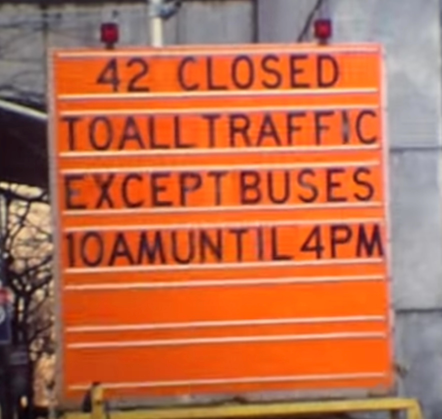
Opening shot from time-lapse video “Transit Day 1990 Auto-Free 42nd Street," filmed on 22 April 1990.
Uploaded to YouTube by Trainluvr, 21 September 2011. Reprinted with permission.
The primary source project Braess’ Paradox in City Planning: An Application of Multivariable Optimization walks the student through a guided reading of excerpts from the 1968 paper “Uber ein Paradoxon aus der Verkehrsplanung” [Braess 1968] (or, in English, “On a paradox of traffic planning” [Braess 2005]) in which this intriguing phenomenon was first studied. Written by Dietrich Braess, currently professor emeritus at Ruhr Universität Bochum, this paper describes a method for detecting this paradox in a network using the framework of combinatorial optimization. When Braess’ paper first appeared, the application of mathematics to traffic planning was still a relatively new idea.1 Today, the paradox that bears his name continues to be studied by mathematical researchers who are interested, for example, in exploring the conditions under which it will not occur. Braess’ paradox is also put to practical use by transportation specialists who are responsible for designing today’s real-life traffic networks. As catalogued by Nagurney & Nagurney [forthcoming], additional applications of Braess’ paradox have been introduced into the modeling of telecommunication networks and the Internet, as well as the study and design of electrical power systems and electronic circuits, mechanical and fluid systems, metabolic networks and ecosystems, and even sports analytics!
Braess' Paradox simulation involving four routes, two of which (in yellow and green) cross the creek bridge.
Observe that the average travel time never exceeds 2 units before the bridge roadblock is removed,
then becomes larger than 2 units once the bridge is opened.
Movie produced by author using the interactive traffic simulator developed by Brian Hayes;
see also [Hayes 2015a, 2015b].
In the student project based on his classic paper, we first retrace Braess' work, and then see how the examples he provided can also be analyzed using standard optimization techniques from a multivariable calculus course. Thus, we provide the student simultaneously with exposure to a second optimization framework and with practice applying the standard multivariable calculus optimization techniques.
The complete project Braess' Paradox in City Planning: An Application of Multivariable Optimization (pdf) is ready for student use, and the LaTeX source code is available from the author by request. A set of instructor notes that explain the purpose of the project and guide the instructor through the goals of each of the individual sections is appended at the end of the student project.
This project is the fifteenth in A Series of Mini-projects from TRIUMPHS: TRansforming Instruction in Undergraduate Mathematics via Primary Historical Sources appearing in Convergence, for use in courses ranging from first-year calculus to analysis, number theory to topology, and more. Links to other mini-PSPs in the series appear below, including four additional mini-PSPs on topics from first-year calculus courses. The full TRIUMPHS collection offers a total of eleven mini-PSPs and one more extensive “full-length” PSP for use with students of calculus.
Note
[1] The first efforts to formulate traffic flow problems mathematically began only in the 1950s, and two publications from that decade [Wardrop 1952, Beckmann et al. 1956] represented the state of the art when Braess himself entered the field. Surprisingly, Braess was completely unaware of those important prior works! His interest in the mathematical modeling of traffic flow instead was inspired by a 1967 seminar talk in which German mathematician W. Knödel presented a certain algorithm that roused Braess’ curiosity. At the time, Braess was 29 years old and had only recently turned to the study of mathematics after completing his doctorate in theoretical physics just three years earlier. Nearly 40 years later, in 2006, Braess delivered his first North American lecture on the paradox named in his honor at the Virtual Center for Supernetworks at University of Massachusetts Amherst. In that lecture, he remarked that both his lack of knowledge of the then-current state of transportation science and his background in physics, which had trained him to look for a counterintuitive symmetry-breaking argument, were important factors in shaping the work that led to his discovery of the paradox that now bears his name.
Acknowledgments
The author would like to thank his advisor Alexander Hulpke and former graduate school classmate Cayla McBee for initial exposure to this wonderful topic! Thanks also to Brian Hayes for creating the simulator which was used to generate the animation above, and for granting permission for its use to produce that animation and to provide a link to the related article Hayes 2015a.
The development of the student project Braess' Paradox in City Planning: An Application of Multivariable Optimization has been partially supported by the TRansforming Instruction in Undergraduate Mathematics via Primary Historical Sources (TRIUMPHS) project with funding from the National Science Foundation’s Improving Undergraduate STEM Education Program under Grants No. 1523494, 1523561, 1523747, 1523753, 1523898, 1524065, and 1524098. Any opinions, findings, and conclusions or recommendations expressed in this project are those of the author and do not necessarily reflect the views of the National Science Foundation. The author gratefully acknowledges this support, with special thanks to TRIUMPHS PI Janet Heine Barnett, who provided assistance with the historical content of the project.
References
Beckmann, Martin J., McGuire, C. B. and Winsten, C. B. 1956. Studies in the Economics of Transportation. New Haven, CT: Yale University Press.
Braess, Dietrich. 1968. Uber ein Paradoxon aus der Verkehrsplanung. Unternehmensforschung 12:258–268.
Braess,Dietrich. 2005. On a Paradox of Traffic Planning. Transportation Science 39(4):446–450. Translation of the original 1968 paper “Uber ein Paradoxon aus der Verkehrsplanung” into English by Anna Nagurney and Tina Wakolbinger.
Hayes, Brian. 2015a. Traffic Jams in Javascript. bit-player blog entry, posted 18 June 2015.
Hayes, Brian. 2015b. Playing in Traffic. American Scientist 103(July–August):260–263.
Kolata, Gina. 1990. What if They Closed 42d Street and Nobody Noticed? New York Times, December 25, 1990, page 38.
Nagurney, Anna and Boyce, David. 2005. Preface to “On a Paradox of Traffic Planning”. Transportation Science 39(4): 443–445.
Nagurney, Anna and Nagurney, Ladimer. ForthThe Braess Paradox. In International Encyclopedia of Transportation, edited by B. Noland, R. Vickerman, and Dick Ettema. Elsevier. Invited chapter, pre-print available at https://supernet.isenberg.umass.edu/articles/braess-encyc.pdf.
Wardrop, John G. 1952. Some Theoretical Aspects of Road Traffic Research. Proceedings of the Institution of Civil Engineers, Part II, 1, no. 2 (August): 325–378.
Completing the Square: From the Roots of Algebra, A Mini-Primary Source Project for Students of Algebra and Their Teachers
Nearly every student of mathematics, after receiving years of training in the rules and procedures of arithmetic, enters the realm of "higher" mathematics through the study of algebraic problem solving, the finding of unknown quantities from known arithmetical conditions on those quantities. Algebra is a staple of the secondary school curriculum around the world, and a standard rite of passage for students in this curriculum is some form of mastery of the process of factoring polynomials, especially quadratic polynomials. Learning to factor quadratics is a precursor to a complete treatment of quadratic equations and their solutions, including the procedure known as "completing the square" and culminating with the well-known quadratic formula: given a quadratic equation of the form \(ax^2+bx+c=0\) (with \(a\neq0\)), its solutions are given by \[x=\frac{-b\pm\sqrt{b^2-4ac}}{2a}.\] The mini-Primary Source Project (mini-PSP) Completing the Square: From the Roots of Algebra presented here is designed to give students a deep understanding of the method of completing the square, which serves as a bridge between the method of factoring and the quadratic formula.
Beginning algebra students naturally focus their attention on mastering the procedures of equation solving and learning to get the correct answers, ignoring questions like "Why and how do the procedures work?" For them, completing the square can involve procedural steps that mysteriously produce the required sought-for answers, and the quadratic formula can act like a runic talisman that magically generates the right numbers that solve the given equation. And even if the question "Why?" is seriously considered in this context, many textbooks answer with a symbolic derivation that is complicated and unsatisfying. The best answer to this question is quite naturally found in the history of the development of this method.
Although problems of quadratic type have been posed and solved for thousands of years, the systematic approach to algebraic problem-solving goes back to the "Father of Algebra," Muḥammad ibn Mūsā al-Khwārizmī (ca 780–850 CE), a ninth-century scholar who wrote in Arabic in the then-young city of Baghdad under the patronage of one of the great caliphs of the Islamic Abbasid Empire. Written in about the year 825, al-Khwārizmī 's extremely influential work on the subject, with the title al-Kitāb al-mukhtaṣar fī hisāb al-jabr wal-muqābala (The Compendious Book on Calculation by Restoration and Reduction), better known today simply as Algebra, instructs his readers how to find the roots of an equation. But al-Khwārizmī's equations are ones without symbols; they are expressed entirely in words. This rhetorical algebra of al-Khwārizmī provides a careful description of the method we call completing the square, along with a clear geometric demonstration of how the method works that involves completing a real (geometric) square!

A page from an Arabic copy of al-Khwārizmī's Algebra,
(https://www.wikiwand.com/en/Muhammad_ibn_Musa_al-Khwarizmi)
In the project Completing the Square: From the Roots of Algebra, students work through selections from al-Khwārizmī's Algebra, using text from two English translations of the work [Rāshid 2009; Rosen 1831]. In a pair of appendices, students can then further explore these ideas through (1) a derivation of the quadratic formula, and/or (2) consideration of when a quadratic equation produces complex roots. The project is meant to serve multiple needs: it can be used by students who are learning algebraic methods for solving quadratic equations for the first time; by future high school mathematics teachers who will be responsible for teaching algebra in their own classrooms; and by students in a general history of mathematics course as an introduction to the role of early Islamic-era mathematics in the development of algebra.
The complete project Completing the Square: From the Roots of Algebra (pdf) is ready for student use, and the LaTeX source code is available from the author by request. A set of instructor notes that explain the purpose of the project and guide the instructor through the goals of each of the individual sections is appended at the end of the student project.
This project is the twelfth in A Series of Mini-projects from TRIUMPHS: TRansforming Instruction in Undergraduate Mathematics via Primary Historical Sources appearing in Convergence, for use in courses ranging from first year calculus to analysis, number theory to topology, and more. Links to other mini-PSPs in the series appear below. The full TRIUMPHS collection also offers dozens of other mini-PSPs and a similar number of more extensive full-length PSPs which are meant for other topics across the undergraduate mathematics curriculum, including a longer version of this project (entitled Solving Equations and Completing the Square: From the Roots of Algebra) that includes an introduction to the rhetorical algebra of al-Khwārizmī and a deeper exploration of his solutions to quadratic equations.
Acknowledgments
The development of the student project Completing the Square: From the Roots of Algebra has been partially supported by the TRansforming Instruction in Undergraduate Mathematics via Primary Historical Sources (TRIUMPHS) project with funding from the National Science Foundation’s Improving Undergraduate STEM Education Program under Grants No. 1523494, 1523561, 1523747, 1523753, 1523898, 1524065, and 1524098. Any opinions, findings, and conclusions or recommendations expressed in this project are those of the author and do not necessarily reflect the views of the National Science Foundation.
References
Katz, Victor, Annette Imhausen, Eleanor Robson, Joseph W. Dauben, Kim Plofker, and J. Lennart Berggren, eds. 2007. The Mathematics of Egypt, Mesopotamia, China, India, and Islam: A Sourcebook. Princeton, NJ: Princeton University Press.
Rāshid, Roshdī. 2009. Al-Khwārizmī: The Beginnings of Algebra. London: Saqi.
Rosen, Frederic. 1831. The Algebra of Moḥammed ben Mūsā, Translated and Edited by Frederic Rosen. London: Oriental Translation Fund.
Connecting Connectedness: A Mini-Primary Source Project for Topology Students
One of the main obstacles for students seeking to understand higher mathematics is the need to grasp a definition. As professional mathematicians, we know that definitions do not fall from the sky, but are instead arrived at through careful and painstaking work. When all is said and done, a good definition is pithy and precise, having been carefully molded with all the right nuances and wording to include the cases we want and to exclude pathologies.
It would seem, however, that this must be news to our students, as the learning of mathematics often begins with a definition rather than ending with it. One of the first places that this traditional pedagogy can begin to cause serious problems for the student is in a first course in topology. A topological space is already a fairly abstract concept, and the properties of topological spaces that one might be interested in studying are even more abstract.
One way to remedy this problem is to trace the evolution of a definition through its historical developments. Although not every definition in topology has a robust historical evolution, one definition with an especially fascinating history is that of connectedness. The concept of connectedness is also one of the more intuitive concepts that is encountered in topology, so that its evolution is quite remarkable to see. This mini-Primary Source Project (mini-PSP), Connecting Connectedness, is an all-too-brief sketch of that evolution.
|
Connectedness was originally defined by Georg Cantor as a condition that a set needed to satisfy in order to constitute a continuum [Cantor 1883]. Two things about Cantor’s definition are especially noteworthy. First, the definition presupposes the existence of a metric. Second, it applies only to closed and bounded sets. In particular, it made no sense for Cantor to ask if the punctured interval \( \, [0,1]-\{{1/2}\}\) was connected. This example becomes a running theme throughout the project, with the question of whether a particular definition can determine that this set is not connected (under the usual topology in \({ R}\), of course) serving as one criterion by which we might judge whether or not we have arrived at a fully satisfactory definition. |
 |
Georg Cantor |
| Camille Jordan (1838–1922). Wikimedia Commons. |
 |
The mini-PSP then looks at the work of Camille Jordan through excerpts from his well-known textbook Cours d’analyse [Jordan 1909]. While Jordan made several contributions to the evolving understanding of the concept of connectedness, the project itself focuses on a specific conceptual distinction that he identified in relation to the concept. Whereas Cantor defined a set to be connected if it satisfied a certain condition, Jordan defined a set to be separated if it satisfied a different condition, and then showed that a set is connected (in Cantor’s sense) if and only if there does not exist a separation. Even though Jordan did not give a new definition of connectedness, his viewpoint of separation as a property of connected sets is the one that we use today. |
|
|
The project’s next primary source comes from [Schoenflies 1904], a work by mathematician Arthur Moritz Schoenflies. Schoenflies had the insight that the concept of distance is not needed to define connectedness. By abstracting away the distance, he then defined the concept in purely point set terms. This was done, in part, to prove that connectedness is a topological invariant (an aspect of Schoenflies’ work that is not covered in the project). | 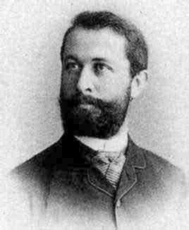 |
Arthur Schoenflies (1853–1928). |
Finally, the project culminates with the work [Lennes 1911] by a Norwegian mathematician who spent his career at Montana State University, Nels Lennes (1874–1951). Lennes was attempting to prove the Jordan Curve Theorem and, in the process, gave the definition of connectedness that we use to this day. Rather than beginning their study of connectedness with the finalized form of the definition, students thus end their project work with that definition. We believe this pedagogy serves our primary goal of building more insight and intuition into the abstract notion of connectedness, as well as our secondary goal of offering students a glimpse into the rich and intriguing history of mathematics.
The complete project Connecting Connectedness (pdf) is ready for student use, and the LaTeX source code is available from the author by request. A set of instructor notes that explain the purpose of the project and guide the instructor through the goals of each of the individual sections is appended at the end of the student project.
This project is the third in A Series of Mini-projects from TRIUMPHS: TRansforming Instruction in Undergraduate Mathematics via Primary Historical Sources appearing in Convergence, for use in courses ranging from first year calculus to analysis, number theory to topology, and more. Links to other mini-PSPs in the series appear below. The full TRIUMPHS collection includes five additional mini-PSPs and two more extensive “full-length” PSPs for use in a topology course, with one of these full PSPs telling the story of the evolution of “connectedness” in greater detail.
Acknowledgments
The development of the student project Connecting Connectedness has been partially supported by the TRansforming Instruction in Undergraduate Mathematics via Primary Historical Sources (TRIUMPHS) project with funding from the National Science Foundation’s Improving Undergraduate STEM Education Program under Grants No. 1523494, 1523561, 1523747, 1523753, 1523898, 1524065, and 1524098. Any opinions, findings, and conclusions or recommendations expressed in this project are those of the author and do not necessarily reflect the views of the National Science Foundation.
References
Cantor, George. 1883. Uber unendliche, lineare Punktmannigfaltigkeiten 5. Mathematische Annalen 21:545–586.
Jordan, Camille. 1893. Cours d'analyse, Volume 1. Paris: Gauthier-Villars.
Lennes, N. J. 1911. Curves in Non-Metrical Analysis Situs with an Application in the Calculus of Variations. American Journal of Mathematics 33(1–4):287–326.
Schoenflies, Arthur. 1904. Beitrage zur Theorie der Punktmengen I. Mathematische Annalen 58:195–238.
Euler's Rediscovery of e: A Mini-Primary Source Project for Introductory Analysis Students
|
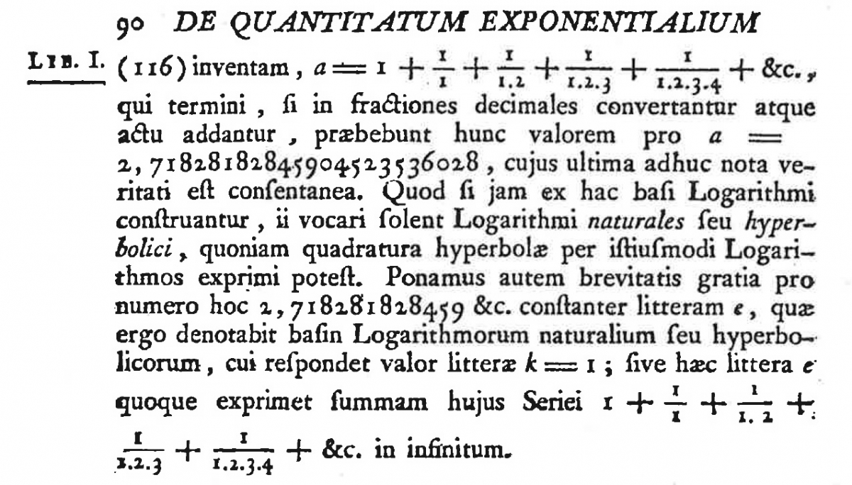
Students meet the celebrated number \(e\) in a number of places in their education, and at various levels of sophistication. This famous constant is used in countless applications and appears periodically in the evolution of mathematics. Leonhard Euler explored \(e\) in his Introductio in Analysin Infinitorum [Euler 1748], one of his most influential works.
|
|

Euler wanted to examine exponential and logarithmic functions, especially as infinite series. Part of his challenge in working with logarithmic functions was to find a logarithmic base for which infinite series expansions are convenient. With this goal in mind, Euler derived \(e\), both as the limiting value of the sequence \(\left( 1+1/j\right) ^{j}\) and as the sum of the infinite series \(1+\dfrac{1}{1}+\dfrac{1}{1\cdot2}+\dfrac{1}{1\cdot2\cdot 3}+\dfrac{1}{1\cdot2\cdot3\cdot4}+\cdots.\) Euler's remarkable development involves clever use of infinitely large and small numbers, which is an aesthetic treat but poses difficult questions for a modern student.
 |
This mini-Primary Source Project, designed for an introductory course in analysis, is structured around passages from Euler's Introductio in Analysin Infinitorum. Students see how \(e\) appears naturally in his development of exponential and logarithmic functions. A vital component of this project is giving a modern justification of \(e=\lim_{j\rightarrow\infty}\left( 1+1/j\right) ^{j}\) using Euler's ideas along with some modern theory. The approach using the Monotone Convergence Theorem, as outlined in project exercises, is a common approach in current analysis textbooks. Reading about it in Euler's own words gives context to the exercises and some appreciation of his dexterity with infinitesimals and series, as well as the close connection with \(e\) as a logarithm base to motivate the definition. Moreover, his series development of \(e^{z}\) is an interesting alternative to the Taylor series approach students have seen in introductory calculus courses.
The complete project Euler's Rediscovery of \(e\) (pdf) is ready for student use, and the LaTeX source code is available from the author by request. A set of instructor notes that explain the purpose of the project and guide the instructor through the goals of each of the individual sections is appended at the end of the student project.
This project is the fifth in A Series of Mini-projects from TRIUMPHS: TRansforming Instruction in Undergraduate Mathematics via Primary Historical Sources appearing in Convergence, for use in courses ranging from first year calculus to analysis, number theory to topology, and more. Links to other mini-PSPs in the series appear below. The full TRIUMPHS collection includes thirteen PSPs for use in a real analysis course.
Acknowledgments
The development of the student project Euler's Rediscovery of \(e\) has been partially supported by the TRansforming Instruction in Undergraduate Mathematics via Primary Historical Sources (TRIUMPHS) project with funding from the National Science Foundation’s Improving Undergraduate STEM Education Program under Grants No. 1523494, 1523561, 1523747, 1523753, 1523898, 1524065, and 1524098. Any opinions, findings, and conclusions or recommendations expressed in this project are those of the author and do not necessarily reflect the views of the National Science Foundation.
References
Euler, Leonard. 1748. Introductio in Analysin Infinitorum, Volume 1. Lausanne: Marcum-Michaelem Bousquet. Also in Euler's Opera Omnia, Series 1, Volume 8, pages 1–392. English translation by John Blanton, 1988, Introduction to Analysis of the Infinite, Book 1, New York: Springer.
Euler’s Calculation of the Sum of the Reciprocals of the Squares: A Mini-Primary Source Project for Calculus 2 Students
A central theme of most second-semester calculus courses is that of infinite series. Students typically learn to classify infinite series as convergent or divergent via a lengthy list of convergence tests. In some cases, they can proceed to evaluate a convergent series by strategically plugging an \(x\) value from the relevant interval of convergence into a power series formula. What is often missing is any indication that it is possible to evaluate an infinite series in any other manner!
Fortunately, in his 1740 paper De Summis Serierum Reciprocarum, Leonhard Euler (1707–1783) provided an example of a nontrivial evaluation of an infinite series that is beautiful and does not require significant extension of the topics one would normally cover in an introductory treatment of power series. Known as The Basel Problem, the evaluation of the series \[\sum_{n=1}^\infty \frac{1}{n^2}=1+\frac{1}{4}+\frac{1}{9}+\frac{1}{16}+\cdots\] proved to be quite a challenge. For example, Jacob Bernoulli (1655–1705) was able to prove the series converged to a number less than \(2\), but the exact value eluded him [Bernoulli 1713]. The mini-Primary Source Project (mini-PSP) Euler's Calculation of the Sum of the Reciprocals of the Squares guides students through Euler's incredibly clever proof that this series converges to \(\pi^2/6\).
Although issues related to series convergence were viewed differently in the 18th century, today's standard series convergence tests are used heavily throughout the project. No prerequisite knowledge is required to understand the proof itself beyond the power series for sine and basics from precalculus such as finding zeros of functions and factoring polynomials. While this project is intended for an introductory calculus course, it also makes an ideal starting point for a discussion of the Riemann zeta function or the Weierstrass Factorization Theorem in a complex analysis course, or a discussion of generating functions in a combinatorics course.
 |
The complete project Euler's Calculation of the Sum of the Reciprocals of the Squares (pdf) is ready for student use, and the LaTeX source code is available from the author by request. A set of instructor notes that explain the purpose of the project and guide the instructor through the goals of each of the individual sections is appended at the end of the student project.
This project is the eleventh in A Series of Mini-projects from TRIUMPHS: TRansforming Instruction in Undergraduate Mathematics via Primary Historical Sources appearing in Convergence, for use in courses ranging from first year calculus to analysis, number theory to topology, and more. Links to other mini-PSPs in the series appear below, including two additional mini-PSPs for first-year calculus. The full TRIUMPHS collection also offers six other mini-PSPs and one more extensive full-length PSP for use with students of calculus.
Acknowledgments
The development of the student project Euler's Calculation of the Sum of the Reciprocals of the Squares has been partially supported by the TRansforming Instruction in Undergraduate Mathematics via Primary Historical Sources (TRIUMPHS) project with funding from the National Science Foundation’s Improving Undergraduate STEM Education Program under Grants No. 1523494, 1523561, 1523747, 1523753, 1523898, 1524065, and 1524098. Any opinions, findings, and conclusions or recommendations expressed in this project are those of the author and do not necessarily reflect the views of the National Science Foundation.
References
Bernoulli, Johanne. 1713. Ars conjectandi, opus posthumum: accedit Tractatus de seriebus infinitis, et epistola Gallice scripta de ludo pil reticularis. Basile: Impensis Thurnisiorum.
Euler, Leonhard. 1740. De summis serierum reciprocarum. Commentarii academiae scientiarum Petropolitanae 7:123–134.
Fermat’s Method for Finding Maxima and Minima: A Mini-Primary Source Project for Calculus 1 Students
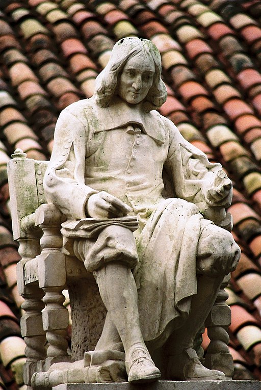
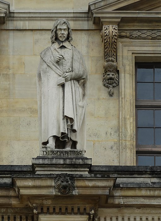
Whether it’s John Adams vs. Thomas Jefferson, or Will Smith vs. Chris Rock, few things capture our attention like a good argument.1 A fantastic example of such a feud arose in the 17th century between two mathematical greats—Pierre de Fermat (1601–1665) and René Descartes (1596–1650)—around a central theme of today’s introductory calculus courses. The mini-Primary Source Project (mini-PSP) Fermat’s Method for Finding Maxima and Minima uses the Fermat vs. Descartes disagreement as an engaging and welcoming point of entry to building a deeper understanding of today’s optimization technique by comparing it with Fermat’s original, more algebraic framework for finding extrema of functions. While students might be initially confused about optimization methods, they don’t need to feel this is an indication that they don’t belong in mathematics: Descartes was flummoxed, too!
 |
 |
|
Statue of Pierre de Fermat by Alexandre Falguière |
Statue of Rene Descartes by Gabriel Garraud, |
As Fermat laid out his method for optimization in his earliest communication of the idea,2 it may sound like some obscure part of the US tax code that only accountants need to know, and then only for their CPA licensing exam. Fermat himself was extremely pleased with his idea,3 declaring that
We can hardly be provided with a more general method.4
Descartes initially dismissed it as nonsense. After reading copies of Fermat's work which Marin Mersenne (1588–1648) passed along to him in 1638, Descartes advised Mersenne that
If . . . he [Fermat] speaks of wanting to send you still more papers, I beg of you to ask him to think them out more carefully than those preceding.5
In the project, students are invited to decode Fermat’s method by trying it out on several of Fermat’s own examples while comparing it, step by step, to the modern method for optimization. The examples themselves are quite short, with the focus placed on understanding the method and its relation to the limit definition of the derivative rather than on attempting to solve challenging optimization problems.6 The optimization problems that Fermat used to demonstrate his method are also very geometric in nature. For instance, the last example featured in the project is the following:
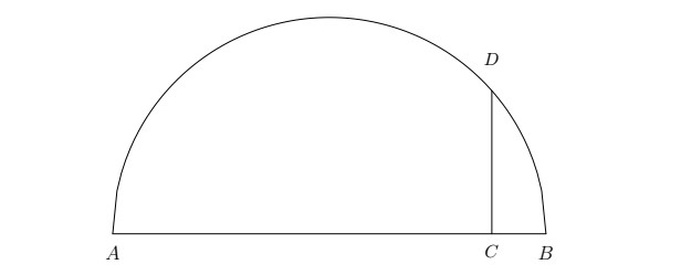
Let there be a semicircle whose diameter is \(AB\); let \(DC\) be perpendicular to it. Find the maximum of the sum of the lines \(AC\) and \(CD\).7
By the end of the project, the student hopefully feels as Descartes finally did when he wrote
Seeing the last method that you use for finding tangents to curved lines, I can reply to it in no other way than to say that it is very good and that, if you had explained it in this manner at the outset, I would have not contradicted it at all.8
The complete project Fermat’s Method for Finding Maxima and Minima (pdf) is ready for student use, and the LaTeX source code is available from the author by request. Instructor notes are provided to explain the purpose of the project and guide the instructor through implementation of the project.
This project is the twenty-sixth in A Series of Mini-projects from TRIUMPHS: TRansforming Instruction in Undergraduate Mathematics via Primary Historical Sources appearing in Convergence, for use in courses ranging from first-year calculus to analysis, number theory to topology, and more. Links to other mini-PSPs in the series appear below. The full TRIUMPHS collection also offers dozens of other mini-PSPs and a similar number of more extensive full-length PSPs. These include an additional twelve mini-PSPs for use in first-year calculus courses as well as four PSPs for use in a multivariable calculus course.
Notes
[1] Especially if it’s John Cleese and Michael Palin, in character!
[2] Here is how Fermat described his method in a missive that was sent to Descartes (by way of Mersennes) in January 1638 (taken from [de Fermat 1636–1642, pp. 133–134]):
Let \(a\) be the desired unknown, whether it be a length, a plane region or a solid, depending on what the given magnitude equals, and let its maximum or minimum be found in terms of \(a\), involving whatever degree. Replace this first quantity with \(a + e\), and the maximum or minimum will be found in terms of \(a\) and \(e\), with coefficients of whatever degree. These two representations of the maximum or minimum are adequated, to use Diophantus’ term, and the common terms are subtracted. Having done this, all terms from either part (affected by e or its powers) are divided each by \(e\), or by a higher power of the same, until some term of one or the other of the expressions is altogether freed from being affected by \(e\).
All terms involving \(e\) or one of its powers are then eliminated and the remaining terms are equated; or, should one of the expressions be left as nothing, then the positive terms are equated with the negatives, which reduces to the same thing. The solution to this last equation will yield the value of \(a\), which will reveal knowledge of the maximum or minimum by referring again to the earlier solutions.
[3] Of course, Fermat’s unique personal style eventually gained him a reputation for coming up with results in secret and then sending them out into the mathematical community with no indication of how one might have come upon that, almost as a puzzle for the world to solve.
[4] Excerpted from [de Fermat 1636–1642, p. 134].
[5] As quoted in [Mahoney 1994, p. 177].
[6] Should the instructor wish to take the students on a longer optimization journey, however, this project would also be the perfect launching point for a student investigation into Snell’s Law, which can be derived from Fermat’s method of optimization.
[7] Excerpted from [de Fermat 1636–1642, p. 153].
[8] As quoted in [Mahoney, 1994, p. 192].
Acknowledgments
The development of the student project Fermat’s Method for Finding Maxima and Minima has been partially supported by the TRansforming Instruction in Undergraduate Mathematics via Primary Historical Sources (TRIUMPHS) Project with funding from the National Science Foundation’s Improving Undergraduate STEM Education Program under Grants No. 1523494, 1523561, 1523747, 1523753, 1523898, 1524065, and 1524098. Any opinions, findings, and conclusions or recommendations expressed in this project are those of the author and do not necessarily reflect the views of the National Science Foundation.
All translations of excerpts from [de Fermat 1636–1642] in this introduction and the mini-PSP were prepared by Daniel E. Otero, Xavier University, 2022. Very minor changes were made by the author to improve readability for the student.
References
de Fermat, Pierre. 1636–1642. Methodus ad disquiredam maxima et minima (Latin). In Oeuvres de Fermat, edited by P. Tannery and C. Henry, Tome 1 (1891), 133–179. French translation in Oeuvres de Fermat, Tome 3 (1896), 121–156. Paris: Gauthier-Villars et fils.
Mahoney, Michael Sean. 1994. The Mathematical Career of Pierre de Fermat, 1601–1665: Second Edition. Princeton, NJ: Princeton University Press.
Fourier's Heat Equation and the Birth of Modern Climate Science: A Mini-Primary Source Project for Differential Equations and Multivariable Calculus Students
The birth of modern climate science is often traced back to the 1827 paper "Mémoire sur les Températures du Globe Terrestre et des Espaces Planétaires" [Fourier 1827] by Jean-Baptiste Joseph Fourier (1768–1830). This work was of course not done in a vacuum, but rather beautifully combined Newton’s Law of Cooling with Euler’s work on differential equations, masterfully uniting ideas from his predecessors. The main ideas had been published five years earlier in Fourier’s groundbreaking study of heat, Théorie analytique de la chaleur [Fourier 1822]. The mini-Primary Source Project (mini-PSP) Fourier’s Heat Equation and the Birth of Climate Science walks the student through key points in that landmark work.
Designed for use in a differential equations course (but also suitable for use in multivariable calculus), the sections of this project tell the following story:
-
Section 1. We see what Fourier’s starting assumptions were for his heat investigation. He essentially began with only Newton’s Law of Cooling!
-
Section 2. We retrace one of Fourier’s primary examples: determining the temperature of a square prism of infinite length. Part of the way through, we find that Fourier snapped his fingers and solved a rather complicated-looking differential equation in just one step.
-
Section 3. The magical incantation he used was some old magic due to Leonhard Euler (1707–1783). In this section, we present this technique in Euler’s own (translated) words, taken from the paper "De integratione aequationum differentialium altiorum graduum” [Euler 1743].
-
Section 4. We return to the infinite square prism problem and apply Euler’s work to confirm Fourier’s solution.
-
Section 5. We present Fourier’s more general heat equation and an intuitive explanation for why it holds.
-
Section 6. We consider Fourier’s solution of the heat problem for an infinite rectangular solid—a geometric object that seems only slightly more complicated than a square prism of infinite length, but for which the century-old algorithm handed to him by Euler couldn’t simply be applied. Instead, Fourier’s work took a very surprising turn as he invented a whole new theory of infinite series, now called Fourier series.
-
Section 7. Finally, students are briefly prompted to explore connections between Fourier’s work and modern climate science.

A graph of the four-term Fourier series expansion of the temperature surface
given by two parallel masses of ice with a mutually-orthogonal hot plate.
Image generated by the author using Geogebra 3D, freely available at https://geogebra.org/3d.
|
The project also provides a short biography of Fourier, who led a truly remarkable life. Born into a working-class family in Auxerre, France, he was orphaned at an early age. From there, he climbed his way all the way up to positions as prominent as the following:
If there were ever an inspiration to students suffering from imposter syndrome as a result of humble origins, it’s Fourier! |
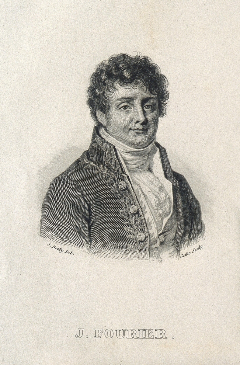 Jean-BaptisteJoseph Fourier. Wellcome Library no. 3110i, public domain. |
The complete project Fourier’s Heat Equation and the Birth of Modern Climate Science (pdf) is ready for student use, and the LaTeX source code is available from the author by request. Instructor notes are provided to explain the purpose of the project and guide the instructor through implementation of the project.
This project is the twenty-second in A Series of Mini-projects from TRIUMPHS: TRansforming Instruction in Undergraduate Mathematics via Primary Historical Sources appearing in Convergence, for use in courses ranging from first-year calculus to analysis, number theory to topology, and more. Links to other mini-PSPs in the series appear below. The full TRIUMPHS collection also offers dozens of other mini-PSPs and a similar number of more extensive full-length PSPs. These include a longer version of this mini-project (entitled Fourier’s Heat Equation and the Birth of Fourier Series) which, in addition to the content described above, takes the student for a joyride with Fourier by following him as he used his trigonometric series to prove a plethora of infinite series identities and briefly exploring how this work served as one impetus to future generations of mathematicians as they explored questions regarding rigor in analysis.
Acknowledgments
The development of the student project Fourier’s Heat Equation and the Birth of Modern Climate Science has been partially supported by the Transforming Instruction in Undergraduate Mathematics via Primary Historical Sources (TRIUMPHS) Project with funding from the National Science Foundation’s Improving Undergraduate STEM Education Program under Grants No. 1523494, 1523561, 1523747, 1523753, 1523898, 1524065, and 1524098. Any opinions, findings, and conclusions or recommendations expressed in this project are those of the author and do not necessarily reflect the views of the National Science Foundation.
References
Euler, Leonhard. 1743. De integratione aequationum differentialium altiorum graduum (On the integration of differential equations of higher orders). Miscellanea Berolinensia, 7:193–242. Eneström number 62. Written in 1742. Reprinted in Opera Omnia: Series 1, Volume 22, pp. 108–149. English translation by Alexander Aycock, Euler Circle-Mainz project, available at https://www.agtz.mathematik.uni-mainz.de/algebraische-geometrie/van-straten/ euler-kreis-mainz.
Fourier, Joseph. 1822. Théorie Analytique de la Chaleur (The Analytical Theory of Heat). Paris: F. Didot. English translation by Alexander Freeman in 1878, Cambridge University Press, Cambridge UK.
Fourier, Joseph. 1827. Mémoire sur les Températures du Globe Terrestre et des Espaces Planétaires (On the Temperatures of the Terrestrial Sphere and Interplanetary Space). Annales de Chimie et de Physique, XXVII:136–167.
Fourier’s Infinite Series Proof of the Irrationality of e: A Mini-Primary Source Project for Calculus 2 Students
|
Three techniques central to the second-semester calculus curriculum are
and
Jean-Baptiste Joseph Fourier's short and beautiful proof that \(e\) is irrational combines exactly these three techniques! |
Jean-Baptiste Joseph Fourier (1768–1830). Wellcome Library no. 3110i, public domain. |
The first written account of Fourier's proof was given by Janot de Stainville (1783–1828), in his Mélanges d’analyse algébrique et de géométrie (Miscellany of algebraic analysis and geometry) [de Stainville 1815, pp. 339–343]. The only idea required to understand this argument that is not typically in the first-year calculus student’s toolbox is that of proof by contradiction. The mini-Primary Source Project (mini-PSP) Fourier’s Infinite Series Proof of the Irrationality of \(e\) introduces the student to this powerful proof technique via a passage from Aristotle and some gentler warm-up contradiction arguments before walking the student through de Stainville’s presentation of Fourier’s lovely argument.
More specifically, the sections of this mini-Primary Source Project entail the following:
-
Section 1 (Proof by Contradiction). In this section, the student learns the general form of a proof by contradiction from a passage in Aristotle’s Prior Analytics [McKeon 1941, 65–107]. A student task then analyzes a simple contradiction argument proving there are infinitely many natural numbers using the well-ordering principle.
-
Section 2 (Some Fundamental Sets of Numbers). Here the project makes sure the student understands exactly what is meant by the words rational and irrational before attempting to prove statements involving these words! The template for an irrationality proof via contradiction is also given.
-
Section 3 (A Warm-up Irrationality Proof). The project returns to the passage from Aristotle, in which he claimed that the side length and diagonal of a square are not commensurate since otherwise “odd numbers are equal to evens.'' The Greek geometers' notions of commensurability/incommensurabilty are briefly related to the rational and irrational numbers.1 The student then works through a proof of the irrationality of \(\sqrt{2}\) corresponding to Aristotle's claim—a much easier warm-up before the main event in the next section!

Raphael, The School of Athens, 1509–1511, fresco at the Raphael Rooms, Apostolic Palace, Vatican City.
Aristotle is depicted in light blue in the center of the fresco standing next to a depiction of Plato in red.
Wikimedia Commons, public domain.
-
Section 4 (Fourier’s Proof of the Irrationality of \(e\)). Here the student works through de Stainville’s argument, which compares the series representation for \(e\) against a geometric series to show that \(e\) is a number between \(2\) and \(3\). Afterwards, the student works through Fourier’s proof by contradiction that proves \(e\) is irrational (as communicated by de Stainville), which again uses a comparison to a geometric series.
-
Section 5 (Transcendence of \(e\)). As a brief epilogue, the student explores the idea of transcendental numbers as an extension of irrationality, comparing the behavior of \(\sqrt{2}\) with that of \(e\).
The project also provides a short biography of Fourier, detailing his inspiring rise from young orphan to prominent mathematician and government official.
The complete project Fourier’s Infinite Series Proof of the Irrationality of \(e\) (pdf) is ready for student use and the LaTeX source code is available from the author by request. Instructor notes are provided to explain the purpose of the project and guide the instructor through its implementation. These notes also provide information about an extended version of this mini-project that instructors seeking a more in-depth experience for their Calculus 2 students may wish to consider [Monks 2022]. The longer project, in which Fourier’s proof of \(e\)’s irrationality is followed up with Joseph Liouville’s (1809–1882) more challenging proof of the irrationality of \(e^2\), is also appropriate for use in an introduction to proofs course or as a part of a capstone experience for prospective secondary mathematics teachers.
This project is the twenty-fifth in A Series of Mini-projects from TRIUMPHS: TRansforming Instruction in Undergraduate Mathematics via Primary Historical Sources appearing in Convergence, for use in courses ranging from first-year calculus to analysis, number theory to topology, and more. Links to other mini-PSPs in the series appear below. The full TRIUMPHS collection also offers dozens of other mini-PSPs and a similar number of more extensive full-length PSPs. These include an additional twelve mini-PSPs for use in first-year calculus courses as well as four PSPs for use in a multivariable calculus course.
Notes
[1] In Section 2 of the extended version of this project (described in the penultimate paragraph of this article), the Greek geometers' notion of commensurate figures is explored in more depth and the student works through a proof of Aristotle's actual claim about the diagonal and the side of a square (albeit using a numerical notion of length and modern symbolism). The definitions of rational and irrational numbers are only given later, in Section 3, where the student is prompted to relate that incommensurabilty proof to the irrationality of \(\sqrt{2}\).
Acknowledgments
The development of the student project Fourier’s Infinite Series Proof of the Irrationality of \(e\) has been partially supported by the TRansforming Instruction in Undergraduate Mathematics via Primary Historical Sources (TRIUMPHS) Project with funding from the National Science Foundation’s Improving Undergraduate STEM Education Program under Grants No. 1523494, 1523561, 1523747, 1523753, 1523898, 1524065, and 1524098. Any opinions, findings, and conclusions or recommendations expressed in this project are those of the author and do not necessarily reflect the views of the National Science Foundation.
References
McKeon, Richard. 1941. The Basic Works of Aristotle. New York: Random House.
Monks, Kenneth M. 2022. Why \(\sqrt{2}\) is Friendlier than \(e\): Irrational Adventures with Aristotle, Fourier, and Liouville. TRIUMPHS Digital Commons Collection. Calculus. 22.
de Stainville, Janot. 1815. Mélanges d’analyse algébrique et de géométrie (Miscellany of algebraic analysis and geometry). Courcier, Paris.
Gaussian Guesswork: Three Mini-Primary Source Projects for Calculus 2 Students
I have begun to examine thoroughly the elastic lemniscatic1 curve depending on \(\int \left (1 – x^4 \right)^{-1/2} dx\).
Gauss’ Mathematical Diary,2 January 8, 1797
At first glance, the integral in this diary entry will look to many students like just another of the possibly hundreds of integrals they encountered in Calculus 2—a course that can seem filled by hours of mundane practice with a dizzying array of techniques and concepts that leave little room for imagination or invention. Hidden from view are the origins of those techniques and concepts in the inventive imaginations of mathematicians such as Carl Friedrich Gauss (1777–1855), for whom the examination of the integral \(\int \left (1 – x^4 \right)^{-1/2} dx\) led to the development of deeply profound and beautiful mathematical results. The three mini-Primary Source Projects (PSPs) presented in this article offer a glimpse of those results within the context of standard techniques and concepts from Calculus 2. Entitled Gaussian Guesswork—and inspired by the article of the same title by Adrian Rice [2009]—each of these three mini-PSPs further offer students an opportunity to witness and experience how experimentation, observation and analogy can play a role in mathematical practice.
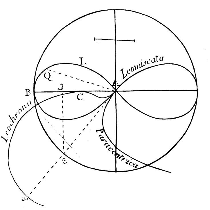
Diagram reproduced from [Bernoulli 1695] showing the lemniscate with the paracentric isochrone.
The curve that Gauss originally called the elastic curve was christened with the name lemniscate by Jacob Bernoulli (1655–1705), in connection with his construction of another curve called the paracentric isochrone. That construction relied on the arclength of the lemniscate, which in turn relies on the very integral that interested Gauss in 1797. In the mini-PSP Gaussian Guesswork: Polar Coordinates, Arc Length and the Lemniscate Curve, students begin by examining the less difficult integral associated with arclengths within the unit circle. Two particular facts about that arclength integral are highlighted:
- \(\int_0^1 \frac{1}{\sqrt{1 – x^2}} dx\) gives the arclength of one-fourth of the unit circle; that is, \(\int_0^1 \frac{1}{\sqrt{1 – x^4}} dx =\frac{\pi}{2}\); and
- the familiar sine function is the inverse of the function defined by \(f(t) = \int_0^t \frac{1}{\sqrt{1 – x^2}} dx\).
After verifying these details through a few preliminary tasks, students are led (again, by way of project tasks) through the process of using polar coordinates to show that the integral for the arclength of one quarter of the unit lemniscate is given by \(\int_0^1 \frac{1}{\sqrt{1 – x^4}} dx\). The project then turns to a brief survey of the conclusions that Gauss derived from the analogy between the two arclength integrals in his paper [Gauss 1797a]; these included:
- the introduction of a new quantity, denoted \(\varpi\) and defined as the arclength of one-fourth of the unit lemniscate; that is, \(\int_0^1 \frac{1}{\sqrt{1 – x^4}} dx=\frac{\varpi}{2}\); and
- the definition of the lemniscatic sine function as the inverse function \(g(t) = \int_0^t \frac{1}{\sqrt{1 – x^4}} dx\).
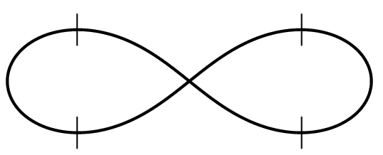
Sketch of the lemniscate from Gauss’ Nachlass [Gauss 1797b, 160].
The numbers \(\pi\) and \(\varpi\) that feature in the mini-PSP described above are two of the three quantities that played a role in Gauss’ guesswork related to the integral \(\int \left (1 – x^4 \right)^{-1/2} dx\). He announced the third quantity in this numerical trio in a later diary entry:
We have established that the arithmetic-geometric mean between \(\sqrt{2}\) and 1 is \(\pi/\varpi\) to 11 places;
the proof of this fact will certainly open up a new field of analysis.
Gauss’ Mathematical Diary, May 30, 1799 (emphasis added)
Gauss appears to have discovered the arithmetic-geometric mean when he was only 14 years old,3 but he published very little about it during his lifetime. The mini-PSP Gaussian Guesswork: Infinite Sequences and the Arithmetic-Geometric Mean draws on a paper that was published posthumously as part of his Nachlass [Gauss 1799]. Students begin this project by reading Gauss’ definition of the two sequences needed to define the arithmetic-geometric mean:4
\[\left \{\begin{array}{cccccccc}a_0, &a_1,&a_2 &a_3, \ldots\\b_0, &b_1,&b_2, &b_3, \ldots\end{array}\right\}\]
. . . [where] the terms of the upper sequence have the value of the arithmetic mean, and those of the lower sequence, the geometric mean:
\[a_1=\frac{1}{2}(a+b), \,\,b_1=\sqrt{ab}, \,\, a_2=\frac{1}{2}(a_1+b_1), \,\,b_2=\sqrt{a_1b_1}, \,\, a_3=\frac{1}{2}(a_2+b_2), \,\,b_3=\sqrt{a_2b_2}. \,\, \]
After working through his first two numerical examples of such sequences and making some observations of their own, students read Gauss’ observations about those same examples and provide proofs of the general properties that he derived from his observations. Here, the Monotone Convergence Theorem arises organically as the natural means to prove the sequences \((a_n)\) and \((b_n)\) are both convergent. The proof that their limits are in fact equal then naturally leads to the definition of the arithmetic-geometric mean between the initial values \(a\), \(b\) as that common limit value.
Gauss’ final example in his Nachlass paper [Gauss 1799] brings in the third number of his numerical trio: the arithmetic-geometric mean between \(\sqrt{2}\) and \(1\).
Example 4: \( a = \sqrt{2}\), \(b = 1\) \[\begin{array}{lll} a_0 \,=\, 1.41421\,35623\,73095\,04880\,2 & \hspace{10pt} & b_0 \, = \, 1.00000\,00000\,00000\,00000\,0 \\ a_1 = 1.20710\,67811\,86547\,52440\,1 & \hspace{10pt} & b_1 = 1.18920\,71150\,02721\,06671\,7\\ a_2 =1.19815\,69480\,94634\,29555\,9 & \hspace{10pt} & b_2 =1.19812\,35214\,93120\,12260\,7\\ a_3= 1.19814\,02347\,93877\,20908\,3 & \hspace{10pt} & b_3 = 1.19814\,02346\,77307\,20579\,8\\ a_4 = 1.19814\,02347\,35592\,20744\,1 & \hspace{10pt} & b_4= 1.19814\,02347\,35592\,20743\,9 \end{array}\]
Here, we see also the reason behind the full title of Rice's article [Rice 2009]:
“Gaussian Guesswork, or why 1.19814023473559220744… is such a beautiful number.”
The mini-PSP Gaussian Guesswork: Elliptic Integrals and Integration by Substitution reveals another connection to this beautiful number by taking up the difficult question of how to evaluate the integral \(\int_0^1 \left (1 – x^4 \right)^{-1/2} dx\) that first sparked Gauss' interest in 1796. The rather surprising result? Letting \(\mu\) denote the arithmetic-geometric mean between \(\sqrt{2}\) and \(1\),
\[\int_0^1 \left (1 – x^4 \right)^{-1/2} dx = \frac{1}{\mu}.\]
Gauss derived this result from a more general integration theorem that he proved in an important astronomical paper on the gravitational attraction of planets [Gauss 1818]. Although the sophisticated substitution that he used in that proof is not itself part of the standard Calculus 2 curriculum, working through its details provides an excellent opportunity for beginning calculus students to apply and consolidate core concepts and techniques while witnessing their interplay within the context of some amazingly beautiful, surprising and important mathematics. Indeed, what began as an examination of a single integral combined with some Gaussian guesswork about a numerical relationship between three numbers not only opened up the field of elliptic functions of a single real-valued variable, but also led Gauss well into the realm of functions of several complex-valued variables and beyond.
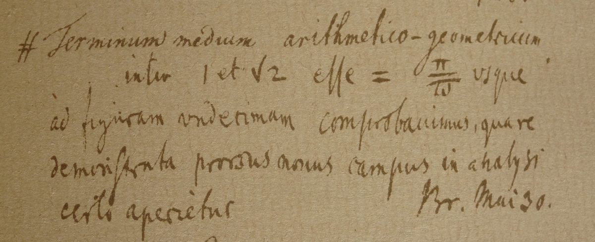
Excerpt from facsimile copy of Gauss’ original diary, from Volume X.1 of Gauss’ Werke.
All three Gaussian Guesswork mini-PSPs are ready for student use:
- Gaussian Guesswork: Polar Coordinates, Arc Length and the Lemniscate Curve (pdf)
- Gaussian Guesswork: Infinite Sequences and the Arithmetic-Geometric Mean (pdf)
- Gaussian Guesswork: Elliptic Integrals and Integration by Substitution (pdf)
Each tells a portion of the tale in some detail, and provides enough of a glimpse of the remaining ideas to give students a feel for the complete story. Any of the three can thus be used either alone or in conjunction with either or both of the others. A set of instructor notes offering practical advice for classroom use is appended at the end of each project. The LaTeX source code of each project is also available from the author by request.
These projects mark the twenty-first entry in A Series of Mini-projects from TRIUMPHS: TRansforming Instruction in Undergraduate Mathematics via Primary Historical Sources appearing in Convergence, for use in courses ranging from first year calculus to analysis, number theory to topology, and more. Links to other mini-PSPs in this series appear below. The full TRIUMPHS collection also offers 10 other mini-PSPs for use in teaching courses in the first-year calculus sequence.
Notes
[1] Originally, Gauss wrote ‘elastic’ here, only to cross it out at some later unknown date when he instead wrote in ‘lemniscatic.'
[2] Gauss’ diary remained in the possession of his family until 1898 and was first published by Felix Klein (1849–1925) in [Klein 1903]. An English translation with commentary on its mathematical contents by the historian of mathematics Jeremy Gray appears in [Gray 1984], and was later reprinted in [Dunnington 2004, 469–496]. A facsimile of the original diary can also be found in Volume X.1 of Gauss’ Werke (Collected Works).
[3] Gauss himself reminisced about his 1791 discovery of this idea in a letter, [Gauss 1816], that he wrote to his friend Heinrich Christian Schumacher (1780–1850) much later. Although his memory of the exact date of his discovery may not have been accurate when he wrote that 1816 letter, Gauss was certainly familiar with the arithmetic-geometric mean by the time he began his mathematical diary in 1796.
[4] Gauss himself used prime notation (i.e., \(a'\), \(a''\), \(a'''\), \(a''''\)) to denote the terms of the sequence. In the project, indexed notation (i.e., \(a_1\), \(a_2\), \(a_3\), \(a_4\)) in keeping with current notational conventions is used instead.
Acknowledgments
The author is grateful to Adrian Rice, whose Math Horizons article “Gaussian Guesswork, or why 1.19814023473559220744 … is such a beautiful number” [Rice 2009] inspired the development of these projects.
The development of the student projects presented in this article has been partially supported by the TRansforming Instruction in Undergraduate Mathematics via Primary Historical Sources (TRIUMPHS) project with funding from the National Science Foundation’s Improving Undergraduate STEM Education Program under Grant No. 1523494. Any opinions, findings, and conclusions or recommendations expressed in this project are those of the author and do not necessarily reflect the views of the National Science Foundation.
References
Bernoulli, Jacob. 1695, December. Explicationes, annotationes et additiones ad ea quæ in Actis superiorum annorum de Curva Elastica, Isochrona Paracentrica, & Velaria, hin inde memorata, & partim controversa lenuntur; ubi de Linea mediarum directionum, aliisque novis (Explanations, notes and additions to that in the Acts of the preceding year about the Elastic, Paracentric Isochrone and Velara Curves, thence from this recounted, the controversial part read, where concerning the line of the middle directions). Acta Eruditorum: 537–553. Also in G. Cramer, editor, Opera Omnia, Volume 1, pages 639–662. Geneva: Cramer, 1744.
Dunnington, Guy Waldo. 2004. Carl Friedrich Gauss: Titan Of Science. Washington, DC: The Mathematical Association of America. Reprint of original 1955 publication. Includes the English translation of Gauss’ Mathematical Diary by Jeremy Gray.
Gauss, Carl Friedrich. 1797a. Elegantiores Integralis \(\int_0^1 \frac{dx}{\sqrt{1 – x^4 }}\) Proprietates (Very Excellent Properties of the Integral \(\int_0^1 \frac{dx}{\sqrt{1 – x^4 }}\)). In Ernst Schering, editor, Werke, volume III, pages 404–412. Göttingen: Gedruckt in der Dieterichschen universitätsdruckerei, 1866.
Gauss, Carl Friedrich. 1797b. Teilung der Lemniskate (Division of the Lemniscate). In Felix Klein, editor, Werke, volume X.1, pages 160–164. Göttingen: Gedruckt in der Dieterichschen universitätsdruckerei, 1917.
Gauss, Carl Friedrich. 1799. Arithmetisch Geometrisches Mittel (Arithmetic-Geometric Mean). In Ernst Schering, editor, Werke, volume III, pages 361–432. Göttingen: Konigliche Gesellschaft der Wissenschaft, 1866.
Gauss, Carl Friedrich. 1816. Letter from Gauss to Schumacher dated April 1816 (in German). In Felix Klein, editor, Werke, volume X.1, pages 247–248. Göttingen: Konigliche Gesellschaft der Wissenschaft, 1917.
Gauss, Carl Friedrich. 1818. Determinatio attractionis, quam in punctum quodvis positionis datae exerceret planeta, si eius massa per totam orbitam ratione temporis, quo singulae partes descibuntur, uniformiter esset dispertita (Determination of the Attraction, which a planet exerts on any point, if its mass is distributed uniformly through the time of the orbit). Presented to the Göttingen Royal Society of Science (January 17, 1818). Also in Ernst Schering, editor, Werke, volume III, pages 331–356. Göttingen: Gedruckt in der Dieterichschen universitätsdruckerei, 1866.
Gray, J. J. 1984. A Commentary on Gauss’s Mathematical Diary, 1796–1814, with an English Translation. Expositiones Mathematicae 2(2):97–130.
Klein, Felix. 1903. Gauss’ Wissenschaftliches Tagebuch (Mathematical Diary), 1796–1814. Mathematische Annalen 57:1–34.
Rice, Adrian. 2009, November. Gaussian Guesswork, or why 1.19814023473559220744 . . . is such a beautiful number. Math Horizons: 12–15.
Generating Pythagorean Triples: A Mini-Primary Source Project in Number Theory for Mathematics Majors, Elementary Teachers and Others
In his commentary on Euclid's proof of the Pythagorean Theorem, Proclus (ca 411–485 CE) asserted [Proclus n.d., pp. 339–340]:
There are two sorts of right-angled triangles, isosceles and scalene. In isosceles triangles you cannot find numbers that fit the sides; for there is no square number that is the double of a square number, if you ignore approximations, such as the square of seven which lacks one of being double the square of five. But in scalene triangles it is possible to find such numbers, and it has been clearly shown that the square on the side subtending the right angle may be equal to the squares on the sides containing it. Such is the triangle in the Republic, in which sides of three and four contain the right angle and five subtends it, so that the square on five is equal to the squares on those sides. For this is twenty-five, and of those the square of three is nine and that of four sixteen. The statement, then, is clear for numbers.
Certain methods have been handed down for finding such triangles, one of them attributed to Plato, the other to Pythagoras.
Although their actual discovery is now hidden in the long shadow of history, the two methods for generating Pythagorean triples described by Proclus remain of interest in number theory today. Proclus’ simple description of how to generate Pythagorean triples using each method offered no speculation about how these algorithms may have been discovered. The mini-Primary Source Project Generating Pythagorean Triples provides students the opportunity to explore how these methods might have become known through an intriguing theory related to the Greek notion of a gnomon.
| With etymological roots in common with the English words gnostic, agnostic and ignorance, the literal meaning of the Greek work gnomon is "that which allows one to know.'' In astronomy, a gnomon is the part of a sundial that casts a shadow, thereby allowing one to know the time. In the ancient world, a vertical stick or pillar often served as the gnomon on a sundial. The term gnomon was also associated in ancient Greek architecture with an L-shaped instrument, sometimes called a 'set square,' that was used for the construction of (or 'knowing of') right angles. |
|
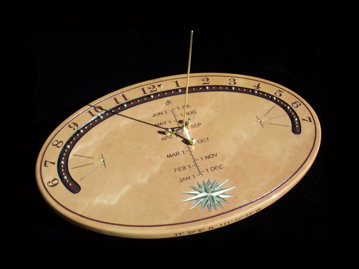
 |
Within Greek mathematics, Euclid used the term gnomon to refer to the plane figure formed by removing any parallelogram from a corner of a larger similar parallelogram. Figure 1 shows the L-shaped gnomon associated with a square. Eventually, Greek mathematicians began to also use the term to refer to the increment between two successive figurate numbers. The square number gnomon diagram shown in Figure 2 is suggested in particular by certain passages in the Physics in which Aristotle (ca 384–ca 322 BCE) discussed the mathematical beliefs of Pythagoras and his followers.
|
|
|


The student project Generating Pythagorean Triples itself begins with an exploration of the primary source excerpt from Proclus above, followed by a brief introduction to the mathematical concept of a gnomon. It then returns to Proclus’ description of the two methods for generating Pythagorean triples which he attributed to Pythagoras and Plato respectively. For each of these two methods, students are presented with a series of tasks. These include numerical tasks based on Proclus' purely verbal descriptions of the two methods, algebraic tasks in which those verbal formulations are translated into symbolic formulas, and geometric tasks that connect the numerical and algebraic formulations of the method in question to gnomons in a figurate number diagram.
Two versions of the project are available, one somewhat more open-ended than the other. Beyond some basic arithmetic and (high school level) algebraic skills, no mathematical content pre-requisites are required in either version. This mini-PSP can thus be used with a wide range of students for whom the study of number theory is part of the curriculum.
Both versions of the project Generating Pythagorean Triples are ready for student use, subtitled The Methods of Pythagoras and of Plato via Gnomons (pdf file) and Gnomonic Explorations (pdf file) respectively. The latter version is the more open-ended, exploratory of the two versions. A set of instructor notes offering practical advice for the use of the project in the classroom is appended at the end of each version. These notes include more detail about the differences between the two versions of the project and the suitability of each for various student audiences. The LaTeX source code of each project is also available from the author by request.
This project is the fourth in A Series of Mini-projects from TRIUMPHS: TRansforming Instruction in Undergraduate Mathematics via Primary Historical Sources appearing in Convergence, for use in courses ranging from first year calculus to analysis, number theory to topology, and more. Links to other mini-PSPs in the series appear below. The full TRIUMPHS collection includes sixteen PSPs for use in courses on number theory.
Acknowledgments
The development of the student projects presented in this article has been partially supported by the TRansforming Instruction in Undergraduate Mathematics via Primary Historical Sources (TRIUMPHS) project with funding from the National Science Foundation's Improving Undergraduate STEM Education Program under grant number 1523494. Any opinions, findings, and conclusions or recommendations expressed in this project are those of the author and do not necessarily represent the views of the National Science Foundation. The author also wishes to thank George W. Heine III for creating the gnomon diagrams in Figures 1 and 2.
References
Proclus. n.d. A Commentary on the First Book of Euclid's Elements. English translation by Glenn R. Morrow, 1970. Princeton, NJ: Princeton University Press.
Henri Lebesgue and the Development of the Integral Concept: A Mini-Primary Source Project for Undergraduate Analysis Students
What classes of functions are integrable? The full answer to this question—that it depends on the type of integration used—is an intriguing fact not generally known to our introductory analysis students.
In the earliest days of calculus, the process of integration was considered to be identical with that of finding an antiderivative. While this meant that any expression that was not itself a derivative could not be integrated, this limitation was neither a theoretical or practical concern at that time. Today, we know that antidifferentiable functions necessarily possess the Intermediate Value Property. This result, known as Darboux's Theorem, rules out integrability for basic step functions under the “integration as antidifferentiation” conception. On the other hand, these discontinuous functions are quite easily integrated under the geometric view of “area under the curve” that emerged as the primary conception of the integral over the course of the 18th century.

Lebesgue's diagram for the Riemann integral.
It was this geometric view of an integral that Cauchy sought to capture by defining the integral as the limit of what is today called a Riemann sum, in tribute to Riemann's thorough investigation of conditions for integrability under that definition. But as Lebesgue noted in the introduction to his doctoral dissertation [Lebesgue 1902]:
It is known that there are derivatives that are not integrable, if one accepts Riemann's definition of the integral; the kind of integration as defined by Riemann does not allow in all cases to solve the fundamental problem of calculus:
Find a function with a given derivative.
It thus seems natural to search for a definition of the integral which makes integration the inverse operation of differentiation in as large a range as possible.
The outcome of Lebesgue's search for such a definition was the integral named in his honor.
The mini-Primary Source Project (PSP) Henri Lebesgue and the Development of the Integral Concept uses excerpts from the relatively non-technical paper “Sur le développement de la notion d’intégrale” [Lebesgue 1927] as a means to consolidate students' understanding of the Riemann integral and its relative strengths and weaknesses. Following a brief overview of the evolution of the integral concept, Lebesgue contrasted the conceptual notions behind the Riemann and Lebesgue integrals. Lebesgue's clever metaphorical comparisons of Riemann's approach to that of an unsystematic merchant “who counts coins and bills at random in the order in which they came to hand,” in contrast to his own approach to that of “a methodical merchant” who stacks coins of the same denomination together before counting them, allowed him to quite naturally bring in the concept of set measure and its role in defining his integral.

Diagram from [Lebesgue 1927] showing the set \(E_i= \{ x \, \vert \, y_i\le f(x) \le y_{i+1}\}\).
In keeping with the content objectives of a typical undergraduate introductory analysis course, the PSP's primary content focus is on the definition and properties of the Riemann integral. Reading about Lebesgue's motivations for developing a different type of integration in his own words also allows students to witness the ways in which mathematicians hone various tools of their trade (e.g., definitions, theorems). The project further touches on issues related to the tensions between “logical rigor” and “geometrical intuition” as guiding principles in mathematics. In fact, Lebesgue explicitly described his new definition of the integral as an effort to reconcile these two desirable but conflicting aspects of mathematics. Additionally, this project offers undergraduates a first (if brief) glimpse of the integral that is the current standard in graduate courses and mathematical research—at least for the time being!
The complete project Henri Lebesgue and the Development of the Integral Concept (pdf) is ready for student use, and the LaTeX source code is available from the author by request. A set of instructor notes that explains the purpose of the project and offers guidance on its implementation is appended at the end of the student project.
This project is the seventh in A Series of Mini-projects from TRIUMPHS: TRansforming Instruction in Undergraduate Mathematics via Primary Historical Sources appearing in Convergence, for use in courses ranging from first year calculus to analysis, number theory to topology, and more. Links to other mini-PSPs in the series appear below. The full TRIUMPHS collection includes thirteen PSPs for use in a real analysis course.
Acknowledgments
The development of the student project Henri Lebesgue and the Development of the Integral Concept has been partially supported by the TRansforming Instruction in Undergraduate Mathematics via Primary Historical Sources (TRIUMPHS) project with funding from the National Science Foundation's Improving Undergraduate STEM Education Program under grant number 1523494. Any opinions, findings, and conclusions or recommendations expressed in this project are those of the author and do not necessarily represent the views of the National Science Foundation. The author also wishes to thank George W. Heine III for recreating the diagrams used in this article.
References
Lebesgue, Henri. 1902. Intégrale, Longueur, Aire. PhD thesis, Université de Paris. Milan: Bernandon de C. Rebeschini.
Lebesgue, Henri. 1927. Sur le développement de la notion d’intégrale. Revue de Metaphysique et de Morale, 34(2):149–167. English translation by Kenneth O. May. In Classics of Mathematics, edited by R. Calinger, 762–765. Prentice-Hall, 1995.
How to Calculate \(\pi\): Buffon's Needle – A Mini-Primary Source Project on Geometric Probability for Calculus 2 Students, Pre-service Teachers and Others
Readers of Convergence are likely to know several ways to calculate \(\pi\). One method—as interesting as it is impractical—can be traced to a 1777 essay by Georges-Louis LeClerc, the Comte de Buffon (1707–1788). The basic idea comes from a question of probability: if a needle of length l is thrown randomly onto a floor marked with parallel lines, set at distance d apart, what is the probability that the needle will cross one of the lines? The lovely answer, calculated by Buffon, is that the probability is precisely \(\frac{1}{\pi}\). While Buffon’s goal was not to calculate \(\pi\), at least one scholar later claimed to have tried to estimate its value using this method. In the mini-Primary Source Project (mini-PSP) How to Calculate \(\pi\): Buffon’s Needle, students examine that claim after first exploring the key ideas from Buffon’s original essay.
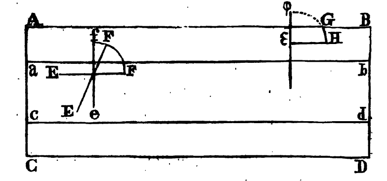
Buffon’s sketch of the Needle Problem.
Beginning shortly before 1750, and continuing until his death in 1788, Buffon published a multi-volume opus, the Histoire Naturelle, which attempted to describe all of nature. To the fourth volume of this work, Discours sur la nature des Animaux, Les Animaux domestiques (Discourse on the nature of Animals: domestic Animals), was appended a “Supplement.” The contents of the supplement give a view into the wide-ranging mind of this natural historian. It contains actuarial tables; additions to already-published articles on childbirth, puberty, the sense of hearing (and many others); replies to scholars who had commented on earlier volumes; and more. Tucked into the middle of all these was a curious work called Essais d’Arithmetique morale (Essays on moral arithmetic) [Buffon 1777].
In a marvelous example of the microcosm reflecting the macrocosm, the Essais has a structure every bit as labyrinthine and fractaline as the larger publication that contains it. In it, Buffon used arguments from what is now known as Utility Theory to argue against gambling; introduced the “Saint Petersburg game” to France; and sought out probabilistic bounds on what it means to be “certain” that an event will occur. Then, just before a philosophical conclusion, he introduced the idea of geometric probability. Although he did not use the term itself, it conveys well his idea that he could ask probabilistic questions that are to be answered geometrically.
Buffon began with the question: If we throw a coin on a floor paved with equal square tiles, and bet as to whether it will fall across a line between two tiles, what size should the tiles be in order for the game to be fair? He concluded that the ratio of the border length to the diameter of the coin should be \(1: 1 - \sqrt\frac{1}{2}\). He then asked the same question for tiles in the form of equilateral triangles, diamonds, and hexagons—stopping when he had exhausted the set of symmetric plane-filling shapes. Next, he made further calculations for each of these shapes, asking about the probability the coin would fall crossing two lines.
Finally, he turned to the question of throwing not a coin, but something one-dimensional (a “needle” or a “baguette”). He replaced the tiles on the floor with parallel lines, and ended up tackling what we now know as “Buffon’s Needle Problem.” Buffon pointed out that in this case, the lack of symmetry meant the problem “would demand a little more geometry.” While he avoided any description of his calculations for the cases described above, he gave enough detail of the needle calculation that the modern reader can follow his work. At the same time, his details are sparse enough—and foreign enough to the modern eye—to necessitate a close and careful read.
This careful read, and an invitation to check details and read between the lines, is the driving force behind the Primary Source Project (PSP) How to Calculate \(\pi\): Buffon’s Needle. Unusually, this project comes in two versions: one suitable for students with no calculus background (but a bit of trigonometry) and one for students who have learned some basic integration. It turns out that most of the creative and clever parts of the geometric probability argument Buffon gave concern carefully setting up the problem, with calculus playing only a minor (if vital) role. Thus calculus students can have the satisfaction of working through the entire argument, which involves evaluating an integral of a trigonometric function using integration by parts. In the non-calculus version, students instead complete Buffon’s argument by looking at the area under a cosine curve, and they are presented with the area value needed to allow them to work through all other details of the mathematics of the problem. Both versions require students to be able to draw a right triangle, label the edges and angles, and write an expression relating some of these using cosine.
The final section of the PSP concerns the famous experiment of Mario Lazzarini, who reported in 1901 that he had conducted an experiment using a floor ruled with parallel lines, and a large set of needles with length equal to \(\frac{5}{6}\) the distance between them [Lazzarini 1901]. He claimed to have thrown these needles on the floor an impressive 3408 times, and he used the number of needles crossing a line to “reverse-engineer” Buffon’s calculations to calculate the value of \(\pi\) based on the experiment. His answer matched the true value to an impressive six decimal places—a feat that seems to have brought Buffon’s Needle Problem out from the obscure text-within-a-text in which it lay to the attention of the wider world. Indeed, a Google Ngrams search of the frequency of occurrence of the phrase “Buffon’s needle” shows a dramatic rise in its use in English-language books starting soon after Lazzarini’s announcement—a rise that shows no evidence of abating (see the graph below). At the same time, his experiment has been viewed with suspicion by later generations, and in the last part of the PSP, students have a chance to engage these suspicions directly.
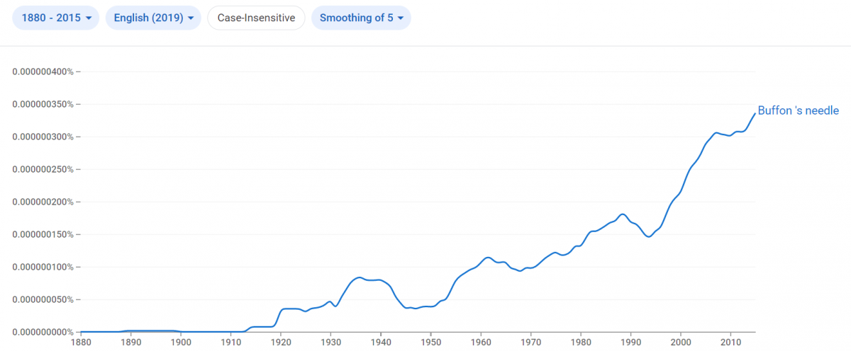
Frequency of occurrence of the phrase “Buffon’s needle” in English language books between 1800 and 2015 (phrase search as case-insensitive, graphs smoothed with a five-year moving average), as provided by Google Ngram Viewer. The growth rate is roughly exponential, with the relative frequency of the phrase in printed English-language books doubling roughly every 30 years since the early 20th century. If left unchecked, the English language will consist of nothing but the words “Buffon’s needle” repeated endlessly by about 2650 CE.
Both versions of the project are ready for student use.
- How to Calculate \(\pi\): Buffon's Needle – Non-calculus version (pdf file)
- How to Calculate \(\pi\): Buffon's Needle – Calculus version (pdf file)
A set of instructor notes that explains the purpose of the project and offers practical advice for classroom use is appended at the end of each project. The LaTeX source code of each project is also available from the author by request.
This project is the twenty-third in A Series of Mini-projects from TRIUMPHS: TRansforming Instruction in Undergraduate Mathematics via Primary Historical Sources appearing in Convergence, which includes a second mini-PSP related to the calculation of \(\pi\):
Links to all mini-PSPs in the series are given below. The full TRIUMPHS collection offers dozens of other mini-PSPs and a similar number of more extensive full-length PSPs, for use in courses ranging from first year calculus to analysis, number theory to topology, and more.
Acknowledgments
The development of the student projects presented in this article has been partially supported by the TRansforming Instruction in Undergraduate Mathematics via Primary Historical Sources (TRIUMPHS) project with funding from the National Science Foundation’s Improving Undergraduate STEM Education Program under Grants No. 1523494, 1523561, 1523747, 1523753, 1523898, 1524065, and 1524098. Any opinions, findings, and conclusions or recommendations expressed in this project are those of the author and do not necessarily reflect the views of the National Science Foundation.
References
Buffon, Comte de (Georges-Louis LeClerc). 1777. Essai d’Arithmétique morale, Supplément à l’Histoire Naturelle, volume 4. Paris: H. Champion.
Lazzarini, Mario. 1901. Un’applicazione del calcolo della probabilita alla ricerca esperimentale di un valore approssimato di \(\pi\). Periodico di Matematica per l'Insegnamento Secondario 4:140–143.
How to Calculate \(\pi\): Machin's Inverse Tangents, A Mini-Primary Source Project for Calculus 2 Students
Almost every mathematical culture through history seems to have proved, trusted, or suspected that the area of a circle is a fixed constant times the square of its radius. It is maybe not surprising, then, that the last two millennia have seen a seemingly endless array of attempts to calculate this constant (today usually called \(\pi\)) with increasing precision. Despite this history, actually calculating \(\pi\) is not a significant part of the standard undergraduate curriculum. (Try asking your senior mathematics majors to calculate \(\pi\) by hand from first principles, even to two decimal places. My own students are not always up to the challenge.)
| Name | Date | Number of Digits |
|---|---|---|
| Archimedes | 250 BCE | 2 |
| Ptolemy | 150 | 3 |
| Liu Hui | 263 | 5 |
| Zu Chongzhi | 480 | 7 |
| Madhava of Sangamagrama | 1400 | 10 |
| Jamshīd al-Kāshī | 1424 | 16 |
| Ludoplh van Ceulen | 1596 | 20 |
| Ludoplh van Ceulen | 1620 | 32 |
| Willebrord Snell | 1621 | 35 |
| Christoph Grienberger | 1630 | 38 |
| Abraham Sharp | 1699 | 71 |
| John Machin | 1706 | 100 |
| Thomas Fantet de Lagny | 1719 | 112 |
| Jurij Vega | 1789 | 126 |
A careful consideration of who has held the record for \(\pi\) calculation at any time is well beyond the scope of this introduction. I would like, however, to accept as a reasonable proxy the list of calculation records as it appears on Wikipedia on the day I write this. (The skeptical reader may like to know that the list is largely consistent with the list on MacTutor.)
It seems that people made progress fairly steadily for 2000 years, as incrementally more effort was spent and better notation was developed. Then, around 1700, progress in digit calculation accelerated noticeably.
|
|
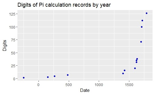
How can we explain this noticeable increase in humanity’s ability to calculate \(\pi\)? It was not the result of simply spending more time and effort on the problem; rather the improvement was a result of a new technology—an understanding of the infinite series of arctangent! One of the first people to put this technology to work was John Machin (1680–1751), a long-time secretary of the British Royal Society.
Machin’s work is fascinating from a modern point of view, as it serves as a bridge between earlier geometric methods of calculating \(\pi\) and the analytic methods based on infinite series that would dominate in the following centuries.
It seems that no record of this work written by Machin himself has survived, but we do have an account of it written by the English judge Francis Maseres (1731–1824), also a Fellow of the Royal Society (Maseres 1796). As Maseres recounted the method, Machin realized he could use the formula for the tangent (or arctangent) of the difference of two angles to estimate a given fraction of \(\pi\), and thus of \(\pi\) itself. In order to do this, Machin needed to find an angle with two important properties:
-
The tangent of the angle is a simple, easy-to-use small fraction; and
-
Using the double-angle formula, one can use this angle to find the tangent of an angle very close to \(\pi\)/4.
As a bonus, it would be nice if plugging the fraction into Leibniz's series led to an easy-to-calculate value.
As some readers of Convergence know, Machin succeeded handsomely in this endeavor. Noting the convenient fact that, in Maseres' words, “the tangent of 1/4 of 45° is nearly = 1/5”, Machin not only knew that
\(\pi/4 ≈ 4 * \arctan(1/5)\),
but was able to use the difference-of-angles formula to find
\(\pi/4 = 4 * \arctan(1/5)\, – \arctan(1/239)\).
A good picture can reveal an entire argument. Segment AB = arctan(1/5), segment AC = 2arctan(1/5), and segment AD = 4arctan(1/5). Angle AMK = \(\pi\)/4, giving us immediately (if we trust the diagram) that \(\pi/4 ≈ 4 * \arctan(1/5)\).
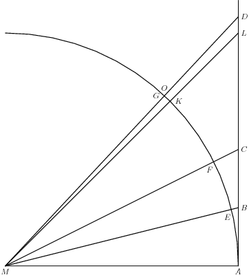
In this Primary Source Project, students use Machin’s ideas about difference-of-tangent formulas and rapidly-converging series to gain an understanding of how \(\pi\) could be calculated. They also gain an appreciation of the relationship between geometric and analytic trigonometry, and can observe directly and numerically how quickly an infinite series (in this case, the Leibniz series for arctangent) converges.
The complete project How to Calculate π: Machin's Inverse Tangents (pdf file) is ready for student use, and the LaTeX source code is available from the author by request. A set of instructor notes that explain the purpose of the project and guide the instructor through the goals of each of the individual sections is appended at the end of the student project.
This project is the sixth in A Series of Mini-projects from TRIUMPHS: TRansforming Instruction in Undergraduate Mathematics via Primary Historical Sources appearing in Convergence, for use in courses ranging from first year calculus to analysis, number theory to topology, and more. Links to other mini-PSPs in the series appear below. An additional three mini-PSPs on methods for calculuating \(\pi\), based on works by Archimedes, Leonhard Euler, and the Compte de Buffon, are also planned for inclusion in the full TRIUMPHS collection.
Acknowledgments
The development of the student project How to Calculate π: Machin's Inverse Tangents has been partially supported by the TRansforming Instruction in Undergraduate Mathematics via Primary Historical Sources (TRIUMPHS) project under Grants No. 1523494, 1523561, 1523747, 1523753, 1523898, 1524065, and 1524098. Any opinions, findings, and conclusions or recommendations expressed in this project are those of the author and do not necessarily reflect the views of the National Science Foundation.
References
Chronology of computation of \(\pi\). Wikipedia. Accessed August 3, 2018.
Maseres, Francis. 1796. A most easy and expeditious method of squaring the circle, invented by the late Mr. John Machin, Professor of Astronomy in Gresham College, London, and Secretary to the Royal Society. Scriptores logarithmici; or a Collection of Several Curious Tracts on the Nature and Construction of Logarithms, Volume III, pp. 155–164. London: J. Davis.
Investigations Into d'Alembert's Definition of Limit: A Mini-Primary Source Project for Students of Real Analysis and Calculus 2
Students of mathematics struggle mightily with the meaning and definition of limit, whether in introductory courses on calculus or in real analysis. This seems fair, since mathematicians themselves have not always agreed on the subtleties of the concept, nor on the need to capture that concept in the form of a precise algebraic definition such as the one that we use today. A major problem in the development of today's definition was finding a useful bridge between the infinitesimal and finite worlds: how to translate ideas like "approach a limiting value" and "as close as we please" into precise algebraic inequalities with clear logical quantifiers. This mini-Primary Source Project (mini-PSP) explores the limit definition given and used by Jean-Baptiste le Rond d'Alembert (1717–1783).
|
|
Early chapters of d'Alembert's biography read like something out of Masterpiece Theater. He was born out of wedlock and left as an infant at the church Saint Jean le Rond in Paris. His salonniére mother Claudine Guérin de Tencin never acknowledged him, and his father Louis-Camus Destouches found another woman to raise young Jean. Destouches died in 1726, but left funds for Jean's education. D'Alembert did well in school and became active as an adult in the philosophy, literature, science and mathematics of his day, standing "at the very heart of the Enlightenment with interests and activities that touched on every one of its aspects" [Hankins 1990]. He co-edited the quintessential work of the French Enlightenment, Diderot’s famous Encyclopédie, for a time, and wrote a number of its articles. Excerpts from two of these, “Limite” and “Calcul différential,” are used in the student project. |

|
There are two versions of this mini-PSP: one for students of real analysis, and a more mild version for use in a first-year calculus course. D'Alembert's definition of limit has pedagogical value for modern students in both courses because it is reasonably close to a verbal version of our modern definition, but with two striking differences. In his 1754 article on the limit [d'Alembert 1754a], d'Alembert asserted (boldface added): One says that a magnitude is the limit of another magnitude, when the second may approach the first more closely than by a given quantity, as small as one wishes, moreover without the magnitude approaching, being allowed ever to surpass the magnitude that it approaches; ...... Strictly speaking, the limit never coincides, or is never equal to the quantity of which it is the limit; but the latter approaches it ever more closely, and may differ from it by as little as one wishes. The circle, for example, is the limit of the inscribed and circumscribed polygons; for strictly it never coincides with them, though they may approach it indefinitely. In other words, d'Alembert did not allow the converging quantity to ever reach or oscillate about the limiting value. Students are confronted with these differences in both versions of the project. |
|
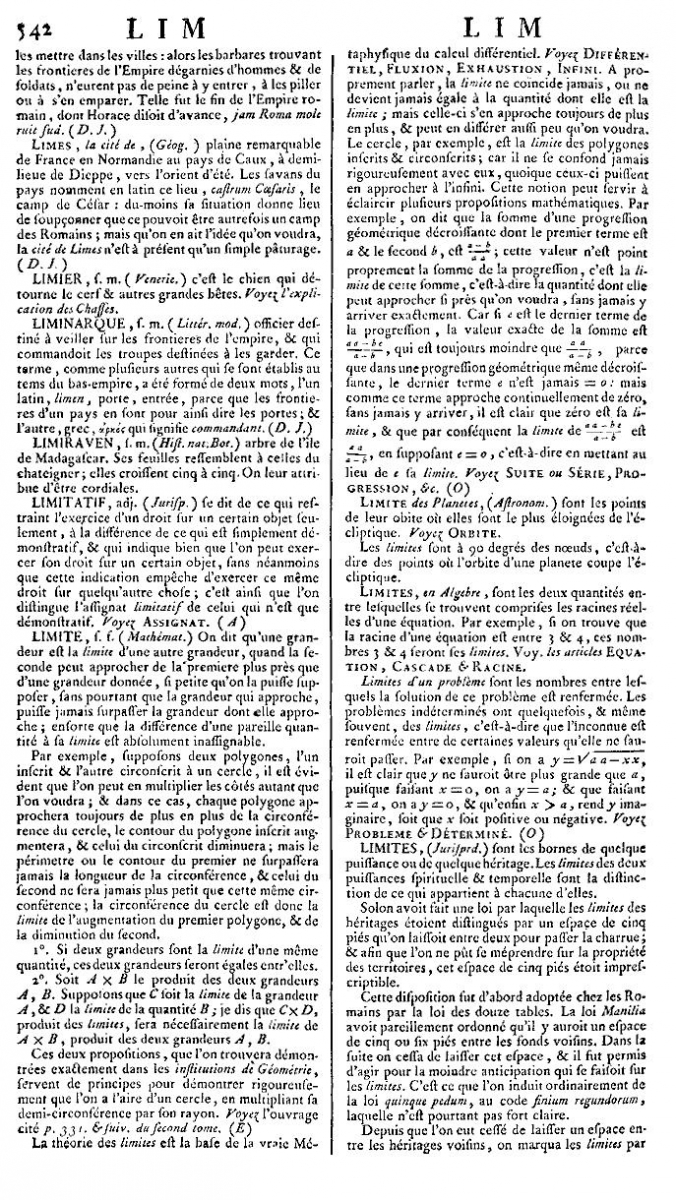
Notably, d'Alembert's example in his 1754 article is sequential in nature, examining sequences of inscribed and circumscribed polygons converging to a circle. After an introduction with some historical background, the mini-PSP also focuses on the limit of a sequence. Some popular textbooks for real analysis treat sequential limits first, so the project can be used as an introduction to this core topic in either course. Proof-related ideas are omitted entirely from the Calculus 2 version of the mini-PSP, which focuses instead on basic examples of sequence convergence. In the real analysis version, students are guided from d'Alembert's verbal description of a sequence limit to a precise modern version using inequalities and quantifiers. That version further investigates two limit properties stated by d'Alembert: uniqueness of limits, and the convergence of a product of two converging quantities. D'Alembert gave a nice proof of the uniqueness result in his “Calcul différential” article, but using phrases such as "approach X as closely as we desire" and "the difference between Y and X can be as small as wished" [D'Alembert 1754b]. Students are asked to translate his theorem statements and give proofs of each in modern language.
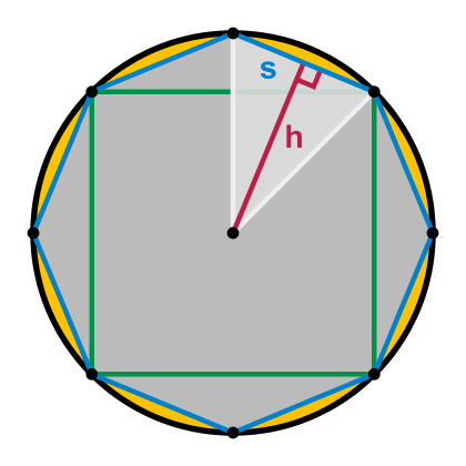
Octagon and square inscribed in circle, showing difference in perimeters.
Created by KSmrq [CC BY-SA (http://creativecommons.org/licenses/by-sa/3.0/)].
Both versions of the project Investigations Into d'Alembert's Definition of Limit are ready for student use, respectively subtitled Real Analysis Version (pdf file) and Calculus 2 Version (pdf file). The LaTeX source code of each is available from the author by request. A set of instructor notes offering background and practical advice for the use of the project in the classroom is appended at the end of both student versions of the project.
This project is the fourteenth in A Series of Mini-projects from TRIUMPHS: TRansforming Instruction in Undergraduate Mathematics via Primary Historical Sources appearing in Convergence, for use in courses ranging from first-year calculus to analysis, number theory to topology, and more. Links to other mini-PSPs in the series appear below. The full TRIUMPHS collection includes twelve PSPs for use in a real analysis course, and seven PSPs for use in a Calculus 2 course.
Acknowledgments
The development of the student projects presented in this article has been partially supported by the TRansforming Instruction in Undergraduate Mathematics via Primary Historical Sources (TRIUMPHS) project with funding from the National Science Foundation’s Improving Undergraduate STEM Education Program under Grants No. 1523494, 1523561, 1523747, 1523753, 1523898, 1524065, and 1524098. Any opinions, findings, and conclusions or recommendations expressed in this project are those of the author and do not necessarily reflect the views of the National Science Foundation. The author gratefully acknowledges this support, with special thanks to TRIUMPHS PI Janet Heine Barnett, who helped with suggestions for producing the Calculus 2 version of the original project.
References
d’Alembert, Jean le Rond. 1754a. Limite (mathématiques). In Encyclopédie ou Dictionnaire raisonné des sciences, des arts et des métiers, volume 9, page 542. Paris. Translation by Jacqueline Stedall, in Mathematics Emerging: A Sourcebook 1540–1900, pp. 297–298, Oxford: Oxford University Press, 2008.
d’Alembert, Jean le Rond. 1754b. Calcul différentiel. In Encyclopédie ou Dictionnaire raisonné des sciences, des arts et des métiers, volume 9, pages 985–988. Paris. Translation by Gregory Bringman, in The Encyclopedia of Diderot & d’Alembert Collaborative Translation Project, Ann Arbor: Michigan Publishing, University of Michigan Library, 2003. https://quod.lib.umich.edu/d/did/did2222.0001.091.
Hankins, Thomas L. 1990. Jean d’Alembert: Science and the Enlightenment. New York: Gordon and Breach.
Lagrange’s Work on Wilson’s Theorem: Three Mini-Primary Source Projects for Number Theory Students
Joseph-Louis Lagrange (1736–1813) enthusiastically began his paper “Proof of a New Theorem Concerning Prime Numbers” [Lagrange 1771] by declaring
I have just found, in an excellent work of Mr. Waring that I recently received, a beautiful arithmetic theorem, which is: If \(n\) is any prime number, the number \(1\cdot 2 \cdot 3 \cdot 4 \cdots (n-1)+1\) will always be divisible by \(n\).
The theorem is known today as Wilson’s Theorem in honor of John Wilson (1741–1793), a student of Edward Waring (1736–1798), who made the observation. Lagrange’s treatment of this beautiful theorem provides a unique opportunity to expose students to two important results of number theory, stated here using modern notation:1
- Wilson’s Theorem: If \(p\) is prime, then \((p-1)! \equiv -1 \pmod{p}\).
- Fermat’s Little Theorem: If \(p\) is prime and \(\gcd(a,p)=1\), then \(a^{p-1} \equiv 1 \pmod{p}\).
His paper is an interesting setting in which to study these results. First, Lagrange presented his proofs in a constructive fashion. That is, he worked through the motivating calculations and presented the results as a consequence. Second, many important number theoretic tools and techniques are used along the way. The three mini-Primary Source Projects (mini-PSPs) presented here take advantage of these pedagogical benefits and Lagrange’s clear writing to guide students through the major highlights of Lagrange’s paper:
- a proof of Wilson’s Theorem that allowed him to deduce Ferma’s Little Theorem as a corollary;
- a proof of the converse of Wilson's Theorem; and
- a proof of Wilson’s Theorem that assumes Fermat’s Little Theorem.
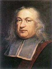
A Trio of Number Theorists: Pierre de Fermat (left, 1601–1665), Joseph-Louis Lagrange (center),
and John Wilson (right). Images courtesy of Convergence Portrait Gallery and Wikipedia.
The mini-PSP Lagrange’s Proof of Wilson’s Theorem—and More presents Lagrange’s first proof of Wilson's Theorem, which he began by comparing the coefficients of the polynomial \[f(x)=(x+1)(x+2)\cdots(x+n-1)\] to those of \(f(x+1)\) using the case of the Binomial Theorem \[(x+1)^n=x^n+nx^{n-1}+\frac{n(n-1)}{2}x^{n-2}+\frac{n(n-1)(n-2)}{2 \cdot 3}x^{n-3}+\dots + nx+1.\] This approach provides a nice illustration of how moving a question from its obvious setting to a larger setting can serve as a powerful problem-solving technique. The main technique in the proof involves solving the system of equations that results from the comparison of these coefficients. Other tools that are used include Euclid's Lemma and the Division Theorem. To prove Fermat’s Little Theorem as a consequence of this approach to Wilson’s Theorem, Lagrange then made a divisibility observation about the polynomial he used in his main proof.
The mini-PSP Lagrange’s Proof of the Converse of Wilson’s Theorem guides students to think carefully about the statement of Wilson’s Theorem, its converse and its contrapositive. Students must also make careful use of quantifiers. While the converse of Wilson’s Theorem does not appear frequently in number theory, the proof itself is pedagogically interesting, especially for students who are relatively new to proof writing. The main number theory tools that appear are about divisibility and the Division Theorem.
In the mini-PSP Lagrange’s Alternate Proof of Wilson’s Theorem students study Lagrange’s second proof of Wilson's Theorem, in which he assumed Fermat’s Little Theorem as a starting point. Modern textbooks often take this approach, but not in the way Lagrange did. Lagrange used the Theory of Differences, that is, a discrete version of differentiation. This is the only part of the three projects that is not common in a modern mathematics curriculum. However, it’s fun, and the necessary explanation and key result, which students are asked to confirm but not prove, are included in the project. Again, divisibility arguments, the Division Theorem, and the Binomial Theorem—here in the form of expanding \((1-1)^n\)—are used.
All three mini-PSPs are ready for student use:
- Lagrange’s Proof of Wilson’s Theorem—and More! (pdf)
- Lagrange’s Proof of the Converse of Wilson’s Theorem (pdf)
- Lagrange’s Alternate Proof of Wilson’s Theorem (pdf)
Each project presents a part of Lagrange’s paper, summarized above in the order in which they appear in Lagrange’s paper. The projects themselves are fully independent of each other and can be used either singly or in combination in any order. A set of instructor notes offering practical advice for classroom use is appended at the end of each project. The LaTeX source of the complete project is also available from the author by request.
These projects mark the twenty-ninth entry in A Series of Mini-projects from TRIUMPHS: TRansforming Instruction in Undergraduate Mathematics via Primary Historical Sources appearing in Convergence, for use in courses ranging from precalculus and first year calculus to analysis, number theory to topology, and more. Links to other mini-PSPs in this series appear below, including the number theory mini-PSPs Generating Pythagorean Triples and The Origin of the Prime Number Theorem. The full TRIUMPHS collection also offers other PSPs (some mini, some not) for use in teaching standard topics in introductory number theory courses, including a project that combines the content of the three mini-PSPs based on Lagrange’s study of Wilson’s Theorem into a single “full-length” PSP.
Acknowledgments
The development of the student projects presented in this article has been partially supported by the TRansforming Instruction in Undergraduate Mathematics via Primary Historical Sources (TRIUMPHS) project with funding from the National Science Foundation’s Improving Undergraduate STEM Education Program under Grants No. 1523494, 1523561, 1523747, 1523753, 1523898, 1524065, and 1524098. Any opinions, findings, and conclusions or recommendations expressed in this project are those of the author and do not necessarily reflect the views of the National Science Foundation.
References
Lagrange, Joseph-Louis. 1771. Démonstration d’un Théorème Nouveau Concernant les Nombres Premiers (Proof of a New Theorem Concerning Prime Numbers). Nouveaux Mémoires de l’Académie Royale des Sciences et Belles-Lettres de Berlin, année 1771, 425–438. Also in Œuveres de Lagrange, Tome 3, pp. 425–440.
[1] The student projects themselves are faithful to Lagrange’s notation and presentation of these theorems.
Regression to the Mean: A Mini-Primary Source Project for Statistics Students
One of the greatest fears in sports performance is that, following a very successful run (of games, shots, field goal kicks, etc.), an individual or team may be “jinxed” and will revert to more average performance. In baseball this has happened so often to second-year players that there is a name for it: the feared “sophomore slump.”
On a seemingly unrelated note ...
Oft-repeated in history books is the lamentation that the progeny of a great man (it does usually seem to be a man in these books) failed to live up to the talent / hard work / brilliance of their parent. The great founding king gives way to a middling prince. Or, in a less regal example, American historian Paul Nagel has described how four generations of the Adams family betrayed an inexorable “Descent from Glory” [Nagel 1990].
Each of these phenomena (from quite unrelated fields) can be explained by the same underlying principle, which is today known as regression to the mean. It states that, given a repeated set of observations, very extreme values will be followed by less extreme ones. This tendency was first noted by Englishman Francis Galton in 1886. Galton seems not only to have been the first person to pose the question of why regression occurs, but in the same paper, he became the first to give an answer. The mini-Primary Source Project Regression to the Mean presented here offers students the opportunity to learn about regression to the mean by reading from his pioneering paper on the topic.
|
Francis Galton (1822–1911) himself is remembered for many things, but for our purposes it may be best to think of him as one of history’s all-time-champion measurers. Nothing that could be quantified escaped his interest, and he was unafraid to use his measurements to draw sweeping conclusions about the world. He studied the lifespan of monarchs and concluded, on the assumption that more people pray for them than pray for average people, that prayer is ineffective in prolonging life. He collected weather data and constructed the first weather map, discovering the phenomenon of “anticyclones” in the process. He even created a “beauty map” of Britain by walking through different cities and making secret records of the attractiveness of women he passed using a device that he called, seemingly with no sense of irony, a “pricker” [Holt 2018]. With an inheritance left to him by his father, Galton gave full rein to his desire to measure things, setting up an “anthropometric laboratory” in London in 1884. He advertised widely, and “thousands of people streamed in and obligingly submitted to measurement of their height, weight, reaction time, pulling strength, color perception, and so on” [Holt 2018, p. 57]. |
|

|
|
In our age of “big data,” many people believe that the company or individual with the best data will have a competitive advantage. More than a century ago, Francis Galton wanted to take many measurements because he believed they would tell him something interesting. Happily, he was correct; with access to an unprecedented amount of anthropometric data, he began to draw conclusions that would otherwise have been impossible, and he thereby became the first person to note the phenomenon of regression. In the Primary Source Project Regression to the Mean, students read parts of Galton’s paper, “Regression Towards Mediocrity in Hereditary Stature” [Galton 1886], to explore the phenomenon and the cause of regression. They are given the opportunity to reason from Galton’s original data of parental and offspring heights, and to explore probabilistic thinking in this setting. Via an optional section of the project, students can also explore errors in reasoning that arise in our world today from a lack of understanding of regression. The complete project Regression to the Mean (pdf) is ready for student use, and the LaTeX source code is available from the author by request. A set of instructor notes that explain the purpose of the project and guide the instructor through the goals of each of the individual sections is appended at the end of the student project. |

This project is the thirteenth in A Series of Mini-projects from TRIUMPHS: TRansforming Instruction in Undergraduate Mathematics via Primary Historical Sources appearing in Convergence, for use in courses ranging from first-year calculus to analysis, number theory to topology, and more. Links to other mini-PSPs in the series appear below, including the statistics mini-PSP Seeing and Understanding Data. The full TRIUMPHS collection also offers a more extensive “full-length” PSP for use in teaching the p-value.
Acknowledgments
The development of the student project Regression to the Mean has been partially supported by the TRansforming Instruction in Undergraduate Mathematics via Primary Historical Sources (TRIUMPHS) project with funding from the National Science Foundation’s Improving Undergraduate STEM Education Program under Grants No. 1523494, 1523561, 1523747, 1523753, 1523898, 1524065, and 1524098. Any opinions, findings, and conclusions or recommendations expressed in this project are those of the author and do not necessarily reflect the views of the National Science Foundation.
References
Galton, Francis. 1886. Regression towards mediocrity in hereditary stature. The Journal of the Anthropological Institute of Great Britain and Ireland 15: 246–263.
Holt, Jim. 2018. Sir Francis Galton, the Father of Statistics … and Eugenics. In When Einstein Walked with Gödel: Excursions to the Edge of Thought, pp. 51–68. New York: Farrar, Straus and Giroux.
Nagel, Paul C. 1999. Descent from Glory: Four generations of the John Adams family. Cambridge: Harvard University Press.
Seeing and Understanding Data: A Mini-Primary Source Project for Students of Statistics
Mathematicians and scientists included drawings in their work before the first statistical graphs were invented. However, their illustrations were meant to depict quantifiable relationships rather than exposing statistical variability. The uses of pictorial representations or charts to convey trends among variable measurements dates back to at least the late 10th century. However, this means of communication did not gain the widespread appreciation it enjoys today until technological advances in the 21st century stimulated the growth of a new field, data visualization. The mini-Primary Source Project (PSP) Seeing and Understanding Data provides students the opportunity to explore the evolution of statistical graphs and visual displays across time and to think critically about how data are displayed and interpreted.
The mini-PSP begins by introducing students to two graphical displays, one from circa 1000 CE (Figure 1) and the other from the mid-15th century (Figure 2), that have features similar to graphs with which they are more familiar. Then, students explore the origins of some now-common statistical graphs in the work of William Playfair (1759–1823), who was apparently the first to publish examples of the pie chart, bar chart, and statistical line chart [Spence & Wainer 2001]. Although Playfair was well-acquainted with major figures of the Scottish Enlightenment, a career checkered by often-illegal activities meant that he and his innovations in communicating data to a general audience remained largely obscure in Great Britain and only slightly better-known in France. It was only in the late 19th century that these graphical methods began to be more widely used by statisticians. (See [Playfair 2005] for a reprint of Playfair’s Commercial and Political Atlas.)
|
|
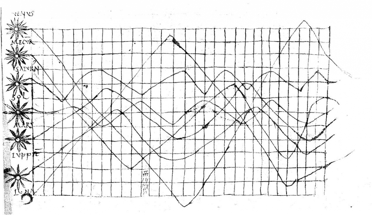
|
|
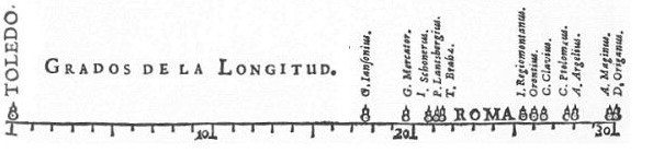
In the 19th century, the professional discipline of statistics and visual representations of data often developed in concert. Graphs came to be used not only to illustrate trends or experiments in science, mathematics, economics, and industry, but also to enhance arguments for social reforms. The mini-PSP explores one such instance, the hand-colored displays Florence Nightingale (1820–1910) prepared for her pivotal report to Britain’s Minister of War to show the proportion of deaths from preventable disease during the Crimean War [Stone 2001]. Her dramatic data displays effected changes to all British Army hospitals—changes also incorporated into the U.S. Army hospitals during the American Civil War. Students investigate both the story and the technical aspects of production for this influential visualization, as well as Charles Minard’s equally elegant display of data from Napoleon’s ill-conceived march on Moscow.
The mini-PSP closes with a look at the production of data displays supported by modern technology. Students then use the nine characteristics of graphical excellence espoused by Edward Tufte (b. 1942) to re-examine the primary source visualizations in the project, including the graphs shown in Figures 1 and 2 above and five other seminal graphs:
-
Exports and Imports of Scotland to and from different parts for one Year from Christmas 1780 to Christmas 1781, Bar Graph by William Playfair
-
Statistical Representation of the United States of America, Pie Chart by William Playfair
-
Chart Shewing the Extent, Population & Revenues, of the Principal Nations of Europe in the Order of their Magnitude, Circle Graph by William Playfair
-
Causes of mortality in the Army in the East, Coxcomb Diagram by Florence Nightingale
-
Successive losses of men in the French Army during the Russian Campaign of 1812–1813, Figurative Map by Charles Joseph Minard
The final project task requires access to the internet (in or out of the classroom) for students to investigate Gapminder’s interactive display of income versus life expectancy data for the whole world over 200 years.
|
|
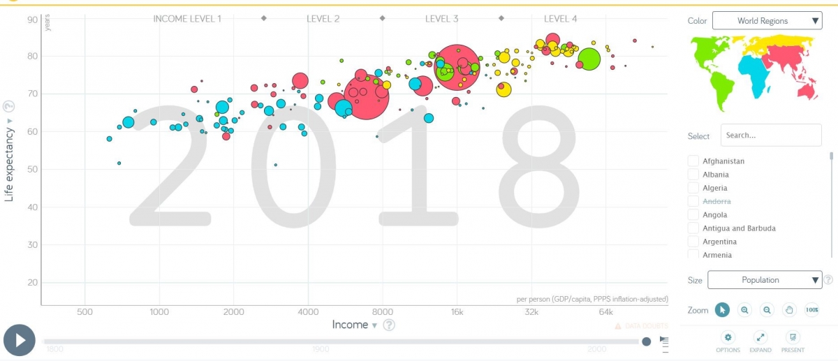
As Hans Rosling once said, “Most of us need to listen to the music to understand how beautiful it is. But often that’s how we present statistics: we just show the notes, we don’t play the music” [Rosling 2007]. Through this mini-PSP, we hope students see and understand how statistical graphs and data visualizations provide the essential music for how statistics is presented and interpreted by the world. Instructors of introductory statistics and data science courses at the high-school and college levels can implement this project over two-three class periods using a combination of small-group work and whole-class discussion. Some project tasks, especially those requiring use of the internet, also work well as individually-assigned out-of-class work. This mini-PSP is also suitable for mathematics education students, and can be completed by middle school students with more assistance and direction from the instructor.
The complete project Seeing and Understanding Data (pdf) is ready for student use and the LaTeX source code is available from the authors by request. Instructor notes are provided to explain the purpose of the project and guide the instructor through each of the individual sections of the project.
This project is the eighth in A Series of Mini-projects from TRIUMPHS: TRansforming Instruction in Undergraduate Mathematics via Primary Historical Sources appearing in Convergence, for use in courses ranging from first year calculus to analysis, number theory to topology, and more. Links to other mini-PSPs in the series appear below. The full TRIUMPHS collection also includes one other PSP for use in teaching statistics, the full-length project entitled Quantifying Certainty: The p-value.
Acknowledgements
The development of the student project Seeing and Understanding Data has been partially supported by the TRansforming Instruction in Undergraduate Mathematics via Primary Historical Sources (TRIUMPHS) project with funding from the National Science Foundation’s Improving Undergraduate STEM Education Program under Grants No. 1523494, 1523561, 1523747, 1523753, 1523898, 1524065, and 1524098. Any opinions, findings, and conclusions or recommendations expressed in this project are those of the author and do not necessarily reflect the views of the National Science Foundation.
References
Anonymous. 1010. De cursu per zodiacum. https://commons.wikimedia.org/wiki/File:Clm_14436_ecliptic_diagram.png#/, accessed November 2, 2018.
Playfair, William. 2005. The Commercial and Political Atlas and Statistical Breviary. Edited and introduced by Howard Wainer and Ian Spence. New York: Cambridge University Press.
Rosling, Hans. 2007, June. Turning Statistics into Knowledge. Paper presented at the Second OECD World Forum on “Statistics, Knowledge and Policy”, Istanbul, Turkey.
Stone, M. 2001. Florence Nightingale. In Statisticians of the Centuries, edited by C. C. Heyde and E. Seneta, 171–175. New York, NY: Springer-Verlag New York, Inc.
Spence, I., and H. Wainer. 2001. William Playfair. In Statisticians of the Centuries, edited by C. C. Heyde and E. Seneta, 105–110. New York, NY: Springer-Verlag New York, Inc.
van Langren, Michaël Florent. 1643. Graph of statistical data, showing the wide range of estimates of the distance in longitude between Toledo and Rome. https://commons.wikimedia.org/wiki/File:Grados_de_la_Longitud.jpg, accessed November 2, 2018.
Solving First-Order Linear Differential Equations: Three Mini-Primary Source Projects for Differential Equations Students
Calculus, and by extension differential equations, has the (earned?) reputation of just being a plethora of seemingly unrelated techniques. Students often try to memorize their way through the course, because it worked when they needed to learn the plethorae (or plethoras) of unrelated facts in other subjects, such as dates or Latin names or chemical elements or vocabulary words or steps in the Krebs cycle. . . . Almost always this ends badly for them.[1] Organizing the different techniques that can be used to solve particular problems is essential to success, and one of the ways to do that is by utilizing history. E. L. Ince (1891–1941) noted that “the historical value of a science depends not upon the number of particular phenomena it can present but rather upon the power it has of coordinating diverse facts and subjecting them to one simple code” [Ince 1926, p. 529]. The three mini-Primary Source Projects (mini-PSPs) in the series Solving First-Order Linear Differential Equations attempt to do exactly that by examining three different techniques—an opaque one-off change of variables, variation of parameters, and exactness with integrating factors—for solving first-order linear differential equations of the form
\[\frac{dy}{dx} +P(x) y = Q(x).\]
Together, the three PSPs follow the historical story of the search for more general methods for solving such equations by examining works due to Gottfried Leibniz (1646–1716), Johann Bernoulli (1667–1748) and Leonhard Euler (1707–1783).

Gottfried Leibniz (left), Johann Bernoulli (center) and Leonhard Euler (right).
Convergence Portrait Gallery.
The first mini-PSP in the series, subtitled Gottfried Leibniz’s ”Intuition and Check” Method, explains how in 1694 Leibniz solved these equations using a one-off method applicable only to this specific problem. Strictly speaking, Leibniz didn’t even solve the equation, but rather asserted a solution and then showed it worked. Part of his proposed solution will be familiar to the students: it is the standard integrating factor method we teach today.
The second project in the series, subtitled Johann Bernoulli’s (Almost) Variation of Parameters Method, explains how in 1697 Bernoulli provided a method for solving Bernoulli differential equations that reduces to variation of parameters when applied to first-order linear equations. This was decades before Lagrange received credit for the technique. Again, part of Bernoulli’s solution will be the standard integrating factor.
The final mini-PSP in the series, subtitled Leonard Euler’s Integrating Factor Method, explains how in 1763 Euler solved these equations as a special case of exact differential equations by finding an integrating factor. His integrating factor is the same as the one the students would have seen. This project is a bit longer than the others, and it may require a bit more time or advance preparation.
The three projects in the series can be utilized individually, or as a trio. They can all be used early in the course when first-order linear differential equations are first covered. Or, they can be spread out through the semester, utilizing the Bernoulli project as an easy motivation when covering variation of parameters and the Euler project when discussing exactness.
The complete projects are ready for student use:
- Solving First-Order Linear Differential Equations: Gottfried Leibniz’s “Intuition and Check” Method (pdf)
- Solving First-Order Linear Differential Equations: Bernoulli’s (Almost) Variation of Parameters Method (pdf)
- Solving First-Order Linear Differential Equations: Leonard Euler’s Integrating Factor Method (pdf)
The LaTeX source is also available from the author by request. Instructor notes are provided to explain the purpose of each project and guide the instructor through implementation of the project.
The projects in this article mark the thirty-first entry in A Series of Mini-projects from TRIUMPHS: TRansforming Instruction in Undergraduate Mathematics via Primary Historical Sources appearing in Convergence, for use in courses ranging from first-year calculus to analysis, number theory to topology, and more. Links to other mini-PSPs in the series, including 15 additional projects for use in introductory calculus courses, appear below. The full TRIUMPHS collection also offers one additional mini-PSP and six more extensive “full-length” PSPs for use in teaching calculus, as well as several projects based on Maria Agnesi’s Instituzioni for use in teaching precalculus.
Acknowledgments
The development of the student projects presented in this article has been partially supported by the TRansforming Instruction in Undergraduate Mathematics via Primary Historical Sources (TRIUMPHS) project with funding from the National Science Foundation’s Improving Undergraduate STEM Education Program under Grants No. 1523494, 1523561, 1523747, 1523753, 1523898, 1524065, and 1524098. Any opinions, findings, and conclusions or recommendations expressed in this project are those of the author and do not necessarily reflect the views of the National Science Foundation.
References
Bernoulli, Johann. 1697. De conoidibus et spaeroidibus quaedam. Solutio analytica æquationis in Actis A. 1695, pag. 553 propositæ (a Fratre Jac. Bernoullio) [On certain conoids and spheroids. An analytic solution to the equation proposed in Acta A., 1695, p. 553 (by my brother, Jacob Bernoulli)]. Acta Eruditorum, Mar. 1697:113–118.
Euler, Leonhard. 1763. De integratione aequationum differentialium (On the integration of differential equations). Novi Commentarii academiae scientiarum Petropolitanae 8:3–63. Reprinted in Opera Omnia, Series 1, Volume 22, pp. 334–394.
Ince, E. L. 1926. Ordinary Differential Equations. London. Reprint, New York: Dover Publications, 1944.
Leibniz, Gottfried. 1694. Letter to l’Hôpital, 27 November 1694. In Mathematische Schriften, Band II, Briefwechsel Zwischen Leibniz, Huygens van Zulichem und dem Marquis de l’Hôspital, edited by C. I. Gerhardt (1850), 255–262. London: D. Nutt.
[1] For example, consider the integral \(\int \frac{x}{1-x^2}dx \). Obviously, we want students to use \(u\)-substitution to attack this problem. However, there is always one student that has memorized “you use trig-substitution when you see \((1-x^2)\).” And perhaps another one who remembers that “when the denominator factors you rewrite as partial fractions” (and still others with more creative, and less correct, cancellations). Unless the techniques are arranged in some order in students’ minds, a one-minute “freebie” problem has turned complicated and stressful. But this problem also gives us the opportunity to place \(u\)-sub, trig-sub and partial fractions in the single context of solving this integral, thereby showing the methods aren’t actually that unrelated.
Solving Linear Higher Order Differential Equations with Euler and Johann Bernoulli: A Mini-Primary Source Project for Differential Equations Students
The first general type of higher order differential equations solved in an undergraduate Ordinary Differential Equations course is homogenous, linear, and with constant coefficients. In other words, equations that can be put in the form \[0 = Ay+ B\frac{dy}{dx} + C\frac{ddy}{dx^2} + D\frac{d^3y}{dx^3} +\dots+ N\frac{d^ny}{dx^n}.\] Historically, this was also the first class to be solved! The mini-Primary Source Project (mini-PSP) Leonhard Euler and Johann Bernoulli Solving Homogenous Higher Order Linear Differential Equations With Constant Coefficients introduces students to that solution technique via excerpts from the correspondence and publications of its discoverer: Leonhard Euler (1707–1783).
On September 15, 1739, Euler wrote a letter to his friend and teacher “the most celebrated esteemed Sir Johann Bernoulli” (1667–1748). Euler corresponded often and with many people. Indeed, more than 2829 letters to and from Euler survive, many containing important results that would be published in the future and that we still use today. But it was in this particular letter that he shared the following discovery.
I have recently found a remarkable way of integrating differential equations of higher degrees in one step, as soon as a finite [algebraic] equation has been obtained. Moreover this method extends to all equations which . . . are contained in this general form:\[y +\frac{A \, dy}{dx}+\frac{B\, ddy}{dx^2}+\frac{C\, d^3 y}{dx^3}+\frac{D\, d^4 y}{dx^4}+\frac{E\, d^5 y}{dx^5} + \text{etc.}=0.\]
As a point of reference, Gottfried Leibniz (1646–1716) published the solution to first order linear differential equations in 1694, almost 50 years earlier. The conversation between Euler and Bernoulli concerning the higher order problem continued through an additional two letters; a December 9, 1739, response from Bernoulli in which he claimed to have been aware of such a result for years, and a January 19, 1740, letter in which Euler provided some additional details of the technique.1 While this correspondence is interesting and informative (and included in this project), the notation is inconsistent and, as Bernoulli complained, the method “lacks a demonstration.”

Portraits of the correspondents: Leonhard Euler (left) and Johann Bernoulli (right).
Convergence Portrait Gallery.
So, we jump a bit into the future. A polished version of the technique was published in Section 12 of Euler’s 1743 article “De integratione aequationum differentialium altiorum graduum” (“On the integration of differential equations of higher orders”) [Euler 1743]. There, he gave a demonstration of the method that any modern student would recognize. He assumed the solutions to the given differential equation have the form \(y=e^{\int p dx}=e^{px}\) and, upon substitution, produced an associated (or auxiliary) algebraic equation. Finding the roots \(p_1, p_2, p_3, \ldots, \) of that algebraic equation then gave rise to the solutions \(e^{p_1 x}, e^{p_2 x}, e^{p_3 x},\ldots\) of the given differential equation. Euler presented his method in four separate cases, taking care to explain how to combine the resulting (linearly independent) solutions to obtain a “complete integral equation" of the given differential equation:
- Distinct real roots of the algebraic equation;
- Repeated roots of the algebraic equation;
- Distinct complex roots of the algebraic equation; and
- Repeated complex roots of the algebraic equation.
This mini-PSP uses the primary sources described above to introduce the technique for solving homogenous higher order linear differential equations with constant coefficients. Euler's presentation of the general method and the cases of distinct and repeated real roots are provided verbatim from the original sources; his description is clear enough to replace any modern treatment. Euler’s justification of the complex cases is also included, but it is different from what we see in today’s textbooks. Thus, it may be pedagogically more helpful to ask students to simply show that the two methods agree, which the project prompts students to do through a series of tasks. Repeated complex roots are also noted (but not emphasized). A “modern” example of each case is provided for students to work through in the initial presentation of each case, with seven additional historical examples drawn from the primary sources supplied in a later section to provide students with further practice. These include “a suitable example" that Euler gave in his 1739 letter to Bernoulli to illustrate his method: the differential equation \(ydx^4 = K^4 d^4 y\), which arises in the study of the vibration of an elastic lamina with one end fixed to a wall (a flat version of the I-beam image shown below). Indeed, on May 5, 1735, Daniel Bernoulli (1700–1782), the son of Johann, wrote to Euler, "For the curve [of the vibrating elastic lamina] I find the equation \(nd^4y = y dx^4\) . . . but this matter is very slippery” (as quoted in [Cannon and Dostrovsky 1981, p. 70]). At that time (4 years before he shared his closed-form solution method with Johann), Euler reported that he was only able to solve this equation in series form, an indication of how slippery the matter actually is.

An elastic I-beam. Animation by Lzyvzl at en.wikipedia, CC BY-SA 3.0, via Wikimedia Commons.
After working through the derivations and examples in the project, we hope students will be able to solve any differential equation of this type (with reasonable auxiliary equation). An historical epilogue to the project offers further context for the problem and the passages that students have read by briefly recounting how Euler's work on this particular class of differential equations led him to consider trigonometry as a study of functions—thereby turning sine and cosine into the trigonometric functions that have since been learned by centuries of high school and college math students!2
The complete project Leonhard Euler and Johann Bernoulli Solving Homogenous Higher Order Linear Differential Equations With Constant Coefficients (pdf) is ready for student use, and the LaTeX source code is available from the author by request. Instructor notes are provided to explain the purpose of the project and to guide the instructor through implementation of the project.
This project is the twenty-fourth in A Series of Mini-projects from TRIUMPHS: TRansforming Instruction in Undergraduate Mathematics via Primary Historical Sources appearing in Convergence, for use in courses ranging from first-year calculus to analysis, number theory to topology, and more. Links to other mini-PSPs in the series appear below. The full TRIUMPHS collection also offers dozens of other mini-PSPs and a similar number of more extensive full-length PSPs. These include six additional projects for use in a differential equations course.
Notes
[1] All three of these letters (and 14 more) were published in their original Latin by Gustaf Eneström (1852–1923) in a series of three articles in the early 20th century. Specific citations for each are as follows:
- September 15, 1739, first letter from Euler [Eneström 1905, pp. 33–38]
- December 9, 1739, Bernoulli response letter [Eneström 1905, pp. 38–43]
- January 19, 1740, return letter from Euler [Eneström 1905, pp. 43–52]
[2] See [Katz 1987] for details of the argument that Euler's recognition of the need for the trigonometric functions as solutions of linear differential equations was the influential factor in his invention of the calculus of those functions.
Acknowledgments
The development of the student project Leonhard Euler and Johann Bernoulli Solving Homogenous Higher Order Linear Differential Equations With Constant Coefficients has been partially supported by the TRansforming Instruction in Undergraduate Mathematics via Primary Historical Sources (TRIUMPHS) project with funding from the National Science Foundation’s Improving Undergraduate STEM Education Program under Grants No. 1523494, 1523561, 1523747, 1523753, 1523898, 1524065, and 1524098. Any opinions, findings, and conclusions or recommendations expressed in this project are those of the author and do not necessarily reflect the views of the National Science Foundation.
References
Cannon, John T., and Sigalia Dostrovsky. 1981. The Evolution of Dynamics: Vibration Theory from 1687 to 1742. New York: Springer-Verlag.
Eneström, Gustaf. 1905. Der Briefwechsel zwischen Leonhard Euler und Johann I Bernoulli [Teil] III, 1739–1746 (The Correspondence between Euler and Johann I Bernoulli Part III, 1739–1746). Bibliotheca Mathematica 6(3):16–87.
Euler, Leonhard. 1743. De integratione aequationum differentialium altiorum graduum (On the integration of differential equations of higher orders). Miscellanea Berolinensia ad incrementum scientiarum 7:193–242. English translation by Alexander Aycock available at the Euler-Kreis Mainz project.
Katz, Victor J. 1987. The Calculus of Trigonometric Functions. Historia Mathematica 14(4):311–324.
The Cantor Set Before Cantor: A Mini-Primary Source Project for Analysis and Topology Students
Historians and others have long suspected that if a mathematical object or theorem is named after a person, then this is all but a guarantee that the object or theorem was not originally due to this person. The study of Pell’s equation goes back about a thousand years before Pell was born. L’Hôpital infamously bought the right to the discovery of the rule now bearing his name from Johann Bernoulli. Burnside’s Lemma is so notorious for having been known before Burnside that it has come to be called "The Lemma that is not Burnside's."
|
|
The Cantor set, named after Georg Cantor (1845–1918), is no exception to this rule. While Cantor defined the set now bearing his name in an 1883 paper, a version of it was defined several years earlier in 1874 by Henry John Stephen Smith in a paper that appeared in the Proceedings of the London Mathematical Society entitled “On the Integration of Discontinuous Functions” [Smith 1874/75]. Smith (1826–1883) was an Irish mathematician and a professor at Oxford. He made significant contributions to number theory as well as analysis, and is best known today for the Smith normal form of a matrix. In his 1875 paper, Smith took up the question of when a discontinuous function can be integrable. While it is easy to find examples of integrable functions which are discontinuous at finitely many points, it is more difficult to construct integrable functions which are discontinuous at infinitely many points. Smith developed a method of constructing such a function. He proved that any function which coincides with an integrable function everywhere other than a nowhere dense set is integrable. He then gave several examples, including a version of the Cantor set, of nowhere dense sets. Applying his theorem, these sets provide examples of integrable functions which are discontinuous on infinitely many points. |
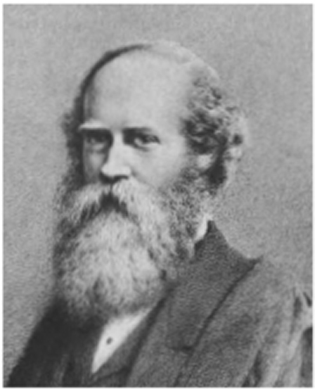
The mini-Primary Source Project (mini-PSP) The Cantor Set Before Cantor begins with the question of how discontinuous a function can be while still being integrable, and ends with the construction of a version of the generalized Cantor set. In the middle of the project, students see Smith’s theorem concerning the construction of integrable functions with discontinuities at every point of a nowhere dense set. After working through some initial definitions and exercises, students are exposed to three of Smith’s examples of nowhere dense sets. The project has the students show that these sets are nowhere dense, and then use Smith’s theorem to construct a function which is discontinuous on that set yet still integrable. Smith’s third example is his version of the Cantor set, a set which illustrates that our initial intuition about how objects “ought” to behave is not always so close to the reality of things. While topologically interesting in its own right, the Cantor set also serves the special purpose of providing an example of an extremely “large” set on which a function can be discontinuous and integrable. In this sense, the project acts as a bridge between analysis and topology that can help students see the connections between the disciplines.

The Cantor set after seven iterations. Wikimedia Commons.
The complete project The Cantor Set Before Cantor (pdf) is ready for student use and the LaTeX source code is available from the author by request. Instructor notes are provided to explain the purpose of the project and guide the instructor through its implementation.
This project is the tenth in A Series of Mini-projects from TRIUMPHS: TRansforming Instruction in Undergraduate Mathematics via Primary Historical Sources appearing in Convergence, for use in courses ranging from first year calculus to analysis, number theory to topology, and more. Links to other mini-PSPs in the series appear below, including the topology mini-PSP Connecting Connectedness. The full TRIUMPHS collection also offers four other mini-PSPs and two more extensive “full-length” PSPs for use in teaching topology.
Acknowledgments
The development of the student projectThe Cantor Set Before Cantor has been partially supported by the TRansforming Instruction in Undergraduate Mathematics via Primary Historical Sources (TRIUMPHS) project with funding from the National Science Foundation’s Improving Undergraduate STEM Education Program under Grants No. 1523494, 1523561, 1523747, 1523753, 1523898, 1524065, and 1524098. Any opinions, findings, and conclusions or recommendations expressed in this project are those of the author and do not necessarily reflect the views of the National Science Foundation.
References
Smith, H. J. S. 1874/75. On the Integration of Discontinuous Functions. Proc. Lond. Math. Soc. 6:140–153.
The Closure Operation as the Foundation of Topology: A Mini-Primary Source Project for Topology Students
As any student of topology will tell you, the main object of study in topology, a topological space, is defined as a set \(X\) along with a collection of subsets of \(X\) satisfying three axioms or properties that concern how unions and intersections of sets behave. The sets in the collection are defined to be “open” sets, a term that is otherwise undefined. This construction is that of the open set axioms. From the open set axioms, one then develops the robust discipline of point-set topology. Many students are also aware of the fact that one can “dualize” the open set axioms by switching the roles of the union and intersection operations, making the necessary adjustments, and defining the sets in this new collection to be “closed.” It is then a helpful but basic exercise to show that these closed set axioms are in fact equivalent to the open set axioms.
What is much less well known among topology students and even topology professors is that the open and closed set axioms are not the only choices for the topological axioms! The mini-Primary Source Project (mini-PSP) The Closure Operation as the Foundation of Topology offers students and their professors an opportunity to explore an equivalent axiomatic system for grounding all of point-set topology based on the work of Polish mathematician and logician, Kazimierz Kuratowski (1896–1980).
|
|
In his foundational textbook Grundzüge der Mengenlehre (Fundamentals of Set Theory), Felix Hausdorff (1868–1942) developed a set of neighborhood axioms [Hausdorff 1914, p. 213]. As part of his 1920 doctoral thesis, Kuratowski developed an equivalent set of axioms using the closure operation. It is with the latter axiomatic system that the project is concerned. While the standard open set axioms are statements about how sets are combined, Kuratowski’s closure axioms are given by essentially defining a function on each set called the closure. This closure function associates to \(A\) a new set \(cl(A)\), denoted \(\overline{A}\) by Kuratowski, that satisfies certain properties. The goal of the project is to show that this closure operation, which on the surface seems to give a very different point of view than the open set axioms, is actually equivalent to the closed set axioms and, consequently, equivalent to the open set axioms. The project begins with an excerpt from the third edition of Hausdorff’s textbook [Hausdorff 1957] in which he discussed the closed set axioms and Kuratowski’s closure axioms. Students then work through excerpts from a 1922 paper by Kuratowski, entitled “Sur l’opération \(\overline{A}\) de l’Analysis Situs” (“On the Closure Operation in Topology”) [Kuratowski 1922], to show that a collection of sets satisfies his closure axioms if and only if it also satisfies the open set axioms.
|
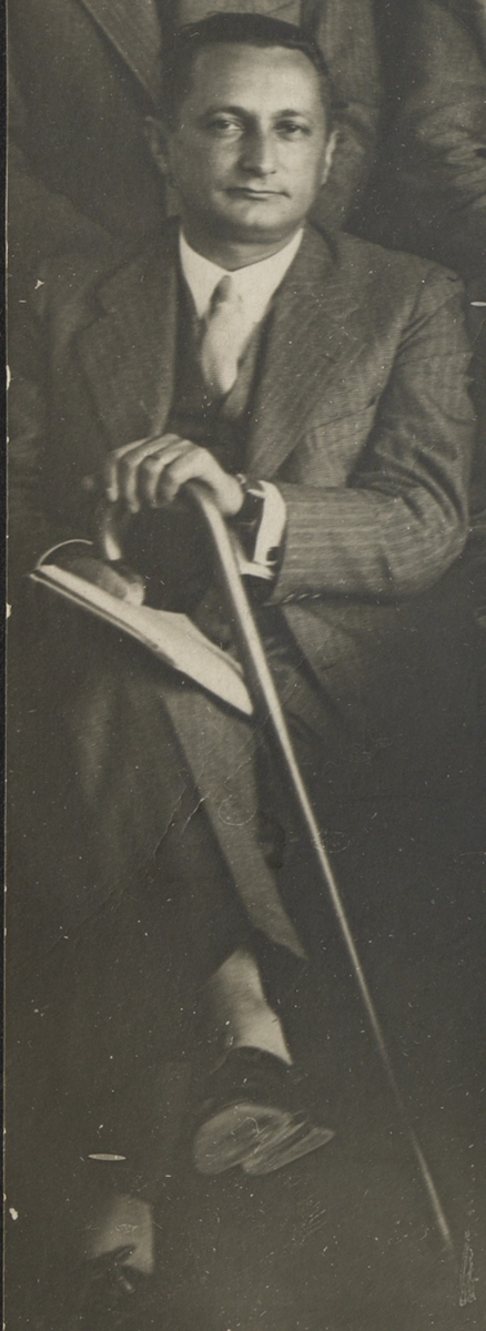
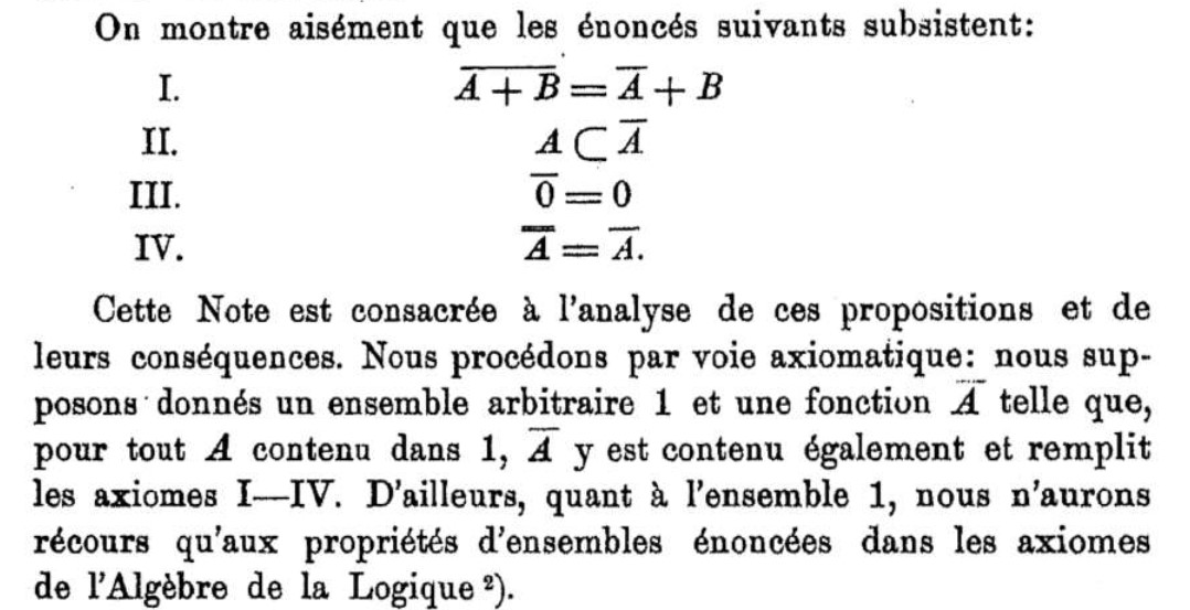
In addition to familiarizing the student with the closure operation, proving the equivalence of the open set axioms with the closure axioms of Kuratowski offers students some key insights about axiomatic systems. First, students see that not only can there be more than one option for an axiomatic system, but axiomatic systems can look very different from one another. Second, students see that geometry isn’t the only branch of mathematics built on a system of axioms (much like how students learn that geometry isn’t the only branch of mathematics that utilizes proof!). As in geometry, a new set of topological axioms allows for generalization and sometimes new branches of mathematics. For example, if one does not require Kuratowski’s closure axiom 3 (as stated in the mini-PSP), one obtains something called a Čech Closure space [Čech 1966] which generalizes many structures and has interesting and important properties [Rieser 2021]. A study of axiomatic systems can thus encourage play and exploration with different, non-equivalent axioms. For if students can create their own geometry and prove theorems from their very own geometric axioms, why can’t they do the same with topology?
The complete project The Closure Operation as the Foundation of Topology (pdf) is ready for student use and the LaTeX source code is available from the author by request. Instructor notes are provided to explain the purpose of the project and guide the instructor through implementation of the project.
This project is the twenty-seventh in A Series of Mini-projects from TRIUMPHS: TRansforming Instruction in Undergraduate Mathematics via Primary Historical Sources to appear in Convergence, for use in courses ranging from first-year calculus to analysis, number theory to topology, and more. Links to other mini-PSPs in the series appear below, including the topology mini-PSPs Connecting Connectedness and Toplogy from Analysis. The full TRIUMPHS collection also offers three other mini-PSPs and two more extensive “full-length” PSPs for use in teaching topology.
Acknowledgments
The development of the student project The Closure Operation as the Foundation of Topology has been partially supported by the TRansforming Instruction in Undergraduate Mathematics via Primary Historical Sources (TRIUMPHS) project with funding from the National Science Foundation’s Improving Undergraduate STEM Education Program under Grants No. 1523494, 1523561, 1523747, 1523753, 1523898, 1524065, and 1524098. Any opinions, findings, and conclusions or recommendations expressed in this project are those of the author and do not necessarily reflect the views of the National Science Foundation.
References
Čech, Eduard. 1966. Topological Spaces. Revised edition by Z. Frolic and M. Katetov. Prague: Publishing House of the Czechoslovak Academy of Sciences; London–New York–Sydney: John Wiley & Sons Interscience Publication.
Hausdorff, Felix. 1914. Grundzüge der Mengenlehre. Leipzig: von Veit.
Hausdorff, Felix. 1935. Mengenlehre. 2nd ed. Leipzig: von Veit. Often identified as the third edition of [Hausdorff 1914].
Hausdorff, Felix. 1957. Set Theory. Providence, RI: AMS Chelsea Publishing, An Imprint of the American Mathematical Society. English translation by John R. Aumann of [Hausdorff 1935].
Kuratowski, Kazimierz. 1922. Sur l’opération \(\overline{A}\) de l’Analysis Situs (On the Closure Operation in Topology). Fundamenta Mathematica 3:182–199.
Rieser, Antonio. 2021, June 1. Čech Closure Spaces: A Unified Framework for Discrete and Continuous Homotopy. Topology and Its Applications, 296: Article 107613, 41 pp.
The Derivatives of the Sine and Cosine Functions: A Mini-Primary Source Project for Calculus 1 Students
This curricular module guides students through a method of calculating the derivative of the sine and cosine functions using differentials. It is based on one primary source: Leonhard Euler's Institutiones calculi differentialis (Foundations of Differential Calculus) [Euler 1755], written in 1748. It was the first calculus book to use functions; indeed, Euler himself had been the first mathematician to regularly use an approach which looks like functions to us today about seven years earlier, in his great "pre-calculus'' book, the Introductio in analysin infinitorum (Introduction to the Analysis of the Infinite) [Euler 1748]. While the use of functions makes the material more accessible to our students today, Euler's approach is different enough from that of modern calculus books that it forces students to think carefully about the material.
 |
The major difference in Euler's approach is the lack of limits in his work. The limit concept would not be formally defined and made a part of mathematics for almost a century; Euler based his calculus (following Leibniz) on the differential dx, which was an infinitely small increment of the variable x. While the logical issues in this approach would force 19th-century mathematicians to abandon it (in favor of limits), Euler saw no such issues. (It is the author's experience that Calculus students are closer to Euler on the epistemological spectrum concerning differentials, and are happy to use them for insight; the author further believes that they provide this insight. Fortunately, this belief will be tested by TRIUMPHS' research component!)
 |
Perhaps the most surprising aspect of Euler's approach is his use of Taylor series. In fact, he introduced these in the Introductio, and thought of them as a pre-calculus idea. In this way, Euler presaged the later work of Lagrange [Lagrange 1797], who used power series as the starting point for his theory of calculus, and defined the derivative as the “first derived function” in the power series expansion of any given function.
This project may be the first time that students see these series, but they do not need any of the theory of Taylor series in the project. The approximations of sine and cosine via three-term Taylor series are presented as a fait accompli, and students are given an opportunity to convince themselves that the approximation seems valid, even if they can't explain why. It is hoped that this exposure will make Taylor series slightly more approachable when they encounter them in the future, but this is not a major goal of the project.
The project The Derivatives of the Sine and Cosine Functions (pdf) is ready for student use, and the LaTeX source code is available from the author by request.
At the end of the project is a set of instructor notes. These echo some of the material in this introduction, and also include practical advice for the use of the project in the classroom.
This project is the first in A Series of Mini-projects from TRIUMPHS: TRansforming Instruction in Undergraduate Mathematics via Primary Historical Sources appearing in Convergence, for use in courses ranging from first year calculus to analysis, number theory to topology, and more. Links to other mini-PSPs in the series appear below. The full TRIUMPHS collection offers additional mini-PSPs and dozens of more extensive full-length PSPs.
Acknowledgments
The development of the student project The Derivatives of the Sine and Cosine Functions has been partially supported by the TRansforming Instruction in Undergraduate Mathematics via Primary Historical Sources (TRIUMPHS) project with funding from the National Science Foundation’s Improving Undergraduate STEM Education Program under Grants No. 1523494, 1523561, 1523747, 1523753, 1523898, 1524065, and 1524098. Any opinions, findings, and conclusions or recommendations expressed in this project are those of the author and do not necessarily reflect the views of the National Science Foundation.
References
Edwards, Harold M. 2007. Euler's definition of the derivative. Bulletin of the American Mathematical Society 44(4): 575–580.
Euler, Leonhard. 1755. Institutiones Calculi Differentialis. St. Petersburg: Academiae Imperialis Scientiarum Petropolitanae. Also in Opera Omnia, Series 1, 10:1–676. English translation by John D. Blanton in Foundations of Differential Calculus, New York: Springer, 2000.
Euler, Leonhard. 1748. Introductio in Analysin Infinitorum. Lausanne: Marcum-Michaelem Bousquet. Also in Opera Omnia, Series 1, 8:1–392. English translation by John D. Blanton in Introduction to Analysis of the Infinite, New York: Springer, 1988.
Lagrange, Joseph-Louis. 1797. Théorie des fonctions analytiques. Paris: Imprimerie de la République.
The Logarithm of −1: A Mini-Primary Source Project for Complex Variables Students
|
By the mid-eighteenth century, logarithms were well understood by European mathematicians. Every positive number had a logarithm, and finding these values had proven useful, both for the pedestrian needs of calculation and to the theoretical development of mathematics. Perhaps it was inevitable that these mathematicians began to ask whether negative numbers also had logarithms—and of all negative numbers, it certainly made sense to start with log(-1). The mini-Primary Source Project (PSP) The Logarithm of -1 provides students with an introduction to the extension of the logarithm function to this new domain, and to the fundamental issues of mathematical “truth” that this extension raises. Deciding whether negative numbers had logarithms at all—and then what the values of these logarithms were—proved a significant challenge to eighteenth-century mathematicians. Among the scholars involved in that debate were Jean le Rond d’Alembert (1717–1783) and Leonhard Euler (1707–1783). It would be difficult to find two more disparate mathematicians. Euler was a devout Christian, a modest and humble man, and one who was perhaps more comfortable with mathematics and the sciences than he was in the company of others. d’Alembert, on the other hand, was the epitome of the humanist French philosophe. He was brilliant, to be sure—among other things, he was one of the leaders of the movement of publish the whole of the world’s knowledge in a grand Encyclopédie (perhaps the best example of a pre-internet Wikipedia), and he worked successfully in fields ranging from history to philosophy.
|
|
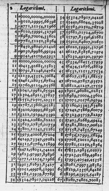
In addition to their vast personal differences, the two men disagreed on a number of mathematical and scientific questions, including the values of the logarithms of negative numbers. One of the most fascinating issues arising from their disagreement is a much larger question: who gets to decide what the value of log(-1) is? Most modern mathematicians would likely agree that some facts from our world are immutable—it’s difficult to imagine, for example, a world in which \(\sqrt{2}\) is rational. Other “facts” generally endorsed by our community of discourse, and taught with authority to our students, are certainly the conscious choice of human definition. For instance, whether the number 1 should be included in the list of prime numbers is clearly a matter of human definition—and experts have come to different verdicts about this question. The early twentieth-century computational number theorist D. H. Lehmer (1905–1991), for example, considered 1 to be prime [Lehmer 1914]. Nearly two thousand years earlier, Nicomachus (60–120) excluded both 1 and 2 from his prime number list.
To which of these categories does the value of log(-1) fall? Does the edifice of existing mathematics force an answer, or are we free to, as it were, use our judgment? This is a delicate kind of question, and it’s one that we don’t often present to our undergraduate students. In contrast, this PSP allows students to glimpse the contingent side of mathematics by following the debate between d’Alembert and Euler as it unfolded, via the original language and thought processes of their time.
It’s worth summarizing the central arguments of the two protagonists here, since both arguments are short and clean. Using the notation of the time, we use “log” to denote the natural logarithm. d’Alembert believed that \(\log(-1)=0\), and he had a few unrelated arguments for why this was so. The most elegant simply applies the existing laws of logarithms and follows them to their natural conclusion. In a letter to Euler (quoted in [Bradley 2007, p. 266]), d'Alembert wrote
All difficulties reduce, it seems to me, to knowing the value of \(\log(-1)\). Now why may we not prove it by the following reasoning? -1 = 1/ -1, so log(-1) = log 1 - log(-1). Thus 2log(-1) = log 1 = 0. Thus log(-1) = 0.
The reader is encouraged to consider this argument, and to see whether they find a flaw in it. (This author confesses he had difficulty finding any such flaws when it was first presented to him.)
|
An easy way to understand Euler’s ideas about this same question (although not the way that he originally expressed them) is to start with that most famous equation \[e^{\pi i} = -1.\] If we accept this, we need only take the natural logarithm of both sides to find that \(\log(-1) = \pi \cdot i\), a value most certainly different than the one d’Alembert proposed. But Euler’s ideas went even further. If we accept (as Euler did) that the equation \[e^{(2n+1)\pi i} = -1\] holds for any integer \(n\), then it would appear that log(-1), paradoxically, takes on the infinitely many different values given by \[\log(-1) = (2n+1)\pi \cdot i. \] |
|

We are returned to our larger question—who is the ultimate arbiter of mathematical truth? In this case, no amount of logic could move either party. In the end, the disagreement between d’Alembert and Euler about this question led to acrimony between the two mathematicians, spilling out into debates about everything from academic precedence to astronomy, and forever tearing asunder a longstanding friendship. While history ultimately declared Leonhard Euler to be the winner, the question of the value of log(-1), and the debate it engendered, still carries lessons for us today.
The complete project The Logarithm of -1 (pdf) is ready for student use and the LaTeX source code is available from the author by request. Instructor notes are provided to explain the purpose of the project and guide the instructor through implementation of the project.
This project is the twentieth in A Series of Mini-projects from TRIUMPHS: TRansforming Instruction in Undergraduate Mathematics via Primary Historical Sources appearing in Convergence, for use in courses ranging from first year calculus to analysis, number theory to topology, and more. Links to other mini-PSPs in this series appear below. The full TRIUMPHS collection also offers one other mini-PSP based on Euler's work along with three more extensive “full-length” PSPs for use in teaching complex analysis.
Acknowledgments
The development of the student project The Logarithm of -1 has been partially supported by the TRansforming Instruction in Undergraduate Mathematics via Primary Historical Sources (TRIUMPHS) project with funding from the National Science Foundation’s Improving Undergraduate STEM Education Program under Grants No. 1523494,1523561, 1523747, 1523753, 1523898, 1524065, and 1524098. Any opinions, findings, and conclusions or recommendations expressed in this project are those of the author and do not necessarily reflect the views of the National Science Foundation.
References
Bradley, R. E. 2007. Euler, D’Alembert and the Logarithm Function. In Leonhard Euler: Life, Work and Legacy, volume 5 of Studies in the History and Philosophy of Mathematics, edited by R. E. Bradley and E. Sandifer, 255–277. Amsterdam: Elsevier.
Lehmer, D. H. 1914. List of Prime Numbers from 1 to 10,006,721. Washington, DC: Carnegie Institution of Washington Publication No. 165.
The Origin of the Prime Number Theorem: A Primary Source Project for Number Theory Students
Near the end of the eighteenth century, Adrien-Marie Legendre (1752–1833) and Carl Friedrich Gauss (1777–1855) seemingly independently began a study of the primes—more specifically, of what we now call their density. It would seem fairly clear to anyone who considered the matter that prime numbers are more rare among larger values than among smaller ones, but describing this difference mathematically seems not to have occurred to anyone earlier. Indeed, there's arguably no a priori reason to assume that there is a nice function that describes the density of primes at all. The mini-Primary Source Project (PSP) The Origin of the Prime Number Theorem provides students with an introduction to this problem through the writing of Gauss and Legendre.
Late in his life (Christmas Day, 1849), Gauss wrote a letter to his colleague Johann Encke (1791–1865) about prime numbers. He reported that he had been interested in primes when he was young, and that in fact he had both tabulated the number of primes in various intervals himself, and then spent some time studying a table of primes that had recently been compiled by Johannn Lambert (1728–1777). As early as 1792 or 1793, Gauss claimed, he had conjectured that the number of primes below a bound \(n\) was, in his notation, \(\int \frac{dn}{\log n}\).
Today we know that Gauss was correct, but we write his conjecture differently. Using more modern notation, and letting as usual \(\pi(x)\) denote the number of primes less than or equal to \(x\), we have
\[\pi(x) \sim \int_2^x \frac{dt}{\log t} \sim \frac{x}{\log x}.\]
(The function \(\mbox{li}(x) = \int_2^x \frac{dt}{\log t} \) is often referred to as the logarithmic integral. The notation \(f(x) \sim g(x)\) indicates that \(\lim_{n \to \infty} \frac{f(x)}{g(x)} = 1\).)
|
|
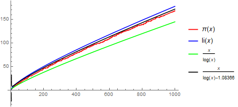
Gauss told no one at the time that he was thinking about prime numbers, and thus Legendre, in the second edition of his Essai sur la Théorie des Nombres (Essay on Number Theory) [Legendre 1808], had good reason to suspect he was the first person to consider the question of the number of primes below a given bound. He began by noting one of the greatest puzzles in modern number theory–the sequence of primes is indeed "extremely irregular," and seems almost random on a small scale, but on a larger scale they seem to follow a rather predictable pattern. Here is how Legendre described this pattern (the English translation is mine):
On a very remarkable law observed in the enumeration of prime numbers
Although the sequence of prime numbers is extremely irregular, one can however find, with a very satisfying precision, how many of these numbers there are from \(1\) up to a given limit \(x\). The formula that resolves this question is
\[y = \frac{x}{\log(x) - 1.08366} \ldots.\]
Legendre then presented a table comparing the values predicted by his formula with the true count, as determined by a recently-published table of primes (Juri Vega's Thesaurus logarithmorum [Vega and Vlack 1794]).
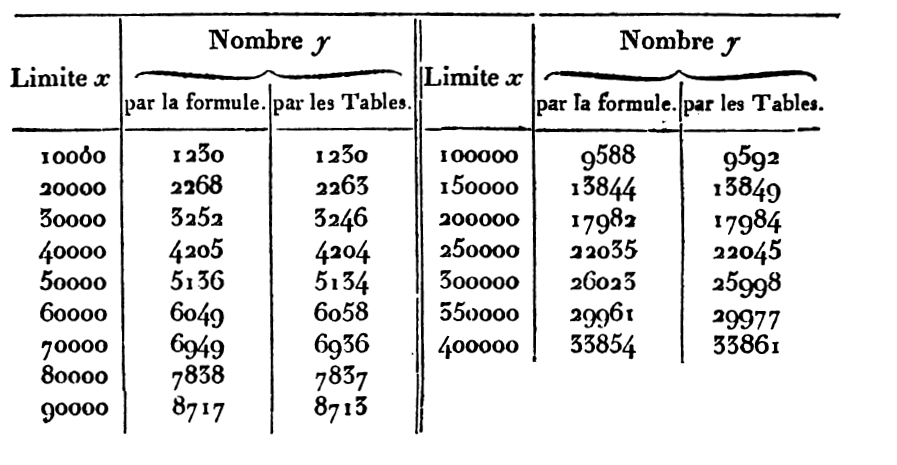
Gauss claimed merely to have looked at the data and seen the pattern; his complete statement reads "I soon recognized that behind all of its fluctuations, this frequency is on the average inversely proportional to the logarithm." Legendre gave even less indication of the origin of his estimate; in particular, his rather precise constant of \(1.08366\) has, as far as I know, never been satisfactorily explained. In the mini-PSP The Origin of the Prime Number Theorem, students explore how Legendre and Gauss may have arrived at their conjectures, compare the similar (though not identical) estimates for the number of primes up to \(x\) given by each, and examine some of the ideas related to different formulations of the Prime Number Theorem. Using the letter written by Gauss, they then examine the error in their respective estimates.
The complete project The Origin of the Prime Number Theorem (pdf) is ready for student use and the LaTeX source code is available from the author by request. Instructor notes are provided to explain the purpose of the project and guide the instructor through implementation of the project.
This project is the ninth in A Series of Mini-projects from TRIUMPHS: TRansforming Instruction in Undergraduate Mathematics via Primary Historical Sources appearing in Convergence, for use in courses ranging from first year calculus to analysis, number theory to topology, and more. Links to other mini-PSPs in the series appear below, including two additional mini-PSPs in number theory. The full TRIUMPHS collection also offers several more extensive “full-length” PSPs for use in teaching number theory.
Acknowledgments
The development of the student project The Origin of the Prime Number Theorem has been partially supported by the TRansforming Instruction in Undergraduate Mathematics via Primary Historical Sources (TRIUMPHS) project with funding from the National Science Foundation’s Improving Undergraduate STEM Education Program under Grants No. 1523494, 1523561, 1523747, 1523753, 1523898, 1524065, and 1524098. Any opinions, findings, and conclusions or recommendations expressed in this project are those of the author and do not necessarily reflect the views of the National Science Foundation.
References
Legendre, Adrien-Marie. 1808. Essai sur la théorie des nombres. 2nd ed. Paris: Courcier.
Vega, George, and Adriaan Vlack. 1794. Thesaurus logarithmorum completus: ex Arithmetica Logarithmeticam, et ex Trigonometria Artificiali Adriani Vlacci collectus, etc. / Vollständige Sammlung Grösserer Logarithmisch-trigonometrischer Tafeln nach Adrian Vlack’s Arithmetica Logarithmetica und Trigonometria Artificialis (Complete collection of logarithmic-trigonometric tables, from the Arithmetica Logarithmica and Trigonometria Artificialis of Adrian Vlack, etc.). Weidmannschen Buchhandlung.
Three Hundred Years of Helping Others: Maria Gaetana Agnesi on the Product Rule – A Mini-Primary Source Project for Calculus 1 Students
If the quantity proposed to be differentiated is the product of several variables, such as \(xy\), whereas \(x\) becomes \(x+dx\), \(y\) becomes \(y+dy\), and \(xy\) becomes \(xy+ydx+xdy+dx\, dy,\) which is the product of \(x+dx\) with \(y+dy\); from this product, then, subtracting the proposed quantity \(xy\), there remains \(ydx+xdy+dx\ dy,\) but \(dx\ dy\) is an infinitely smaller quantity than each of the other two, which are the rectangle of a finite quantity with an infinitesimal, and \(dx \, dy\) is the rectangle of two infinitesimals, and therefore infinitely smaller, so this rectangle can frankly be neglected, therefore the differential of \(xy\) will be \(xdy+ydx\). [Agnesi 1748, p. 458].1
By the mid-eighteenth century, many of the ideas of what we today call calculus existed in some form, but the subject was still in its early stages of development. The state of the literature in particular attested to this: related results based on different underlying ideas were scattered throughout countless publications in different languages and printed in different countries. Luckily for the students of that era, a herculean, benevolent effort was underway. The expository genius Maria Gaetana Agnesi (1718–1799) was hard at work on her two-volume book Instituzioni Analitiche ad Uso della Gioventú Italiana (Foundations of Analysis for Use of the Italian Youth) with the aim of making accessible to the many knowledge that had previously been held only by the few.2 Not only did Agnesi’s book offer a complete introductory treatment of precalculus, differential calculus, and integral calculus in a single work, it was also one of the first calculus textbooks written in a vernacular language instead of Latin. The mini-Primary Source Project (mini-PSP) Three Hundred Years of Helping Others: Maria Gaetana Agnesi on the Product Rule enables today’s students and teachers to benefit from this marvelous work, just as those of the eighteenth century did.
|
|
|
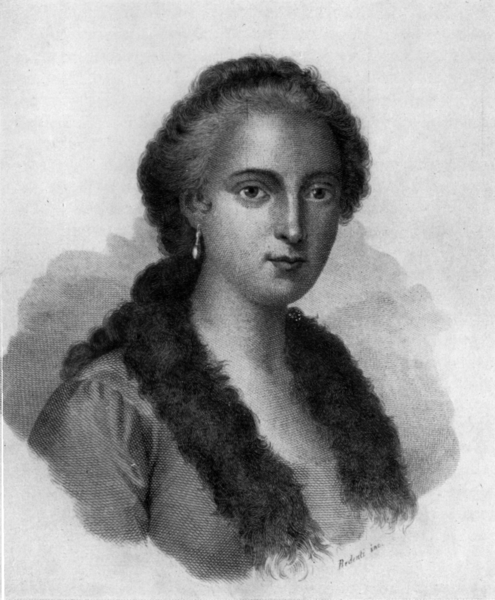
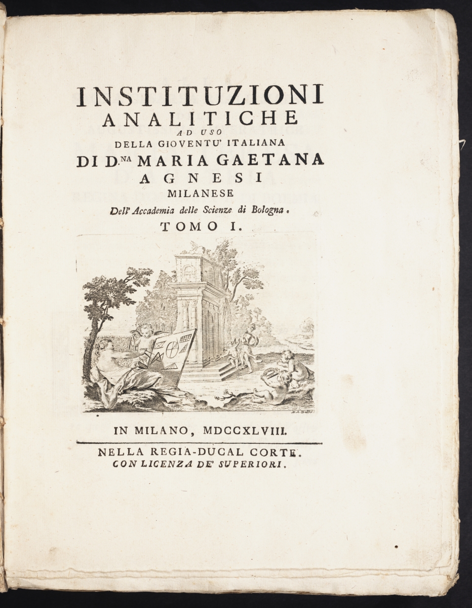
Specifically, this mini-PSP visits the standard single-variable calculus topic of differentiation rules. While students often become adept at applying these rules through drilling, it is rare that today's standard framework of defining the derivative via a limit of a difference quotient provides them with much intuition with regards to these rules. At its worst, the somewhat mysterious difference quotient approach can lead to errors of the “derivative of the product is the product of the derivatives” variety. Agnesi’s treatment of the product rule offers an alternative framework for justifying the correct rule that may have a better chance of sticking with a first-semester calculus student. In particular, the differential explanation that she gave in the above quotation lends itself to a more visual—and thus for many of our students, more intuitive—justification of the product rule.

Through the project tasks, students interpret Agnesi's words as quoted at the top of this page using the labeled geometric diagram shown above, thus deriving the basic product rule. As Agnesi proceeded to extend her approach to products of three quantities [Agnesi 1748, p. 459], the mini-PSP does the same by inviting students to deduce the product rule for three factors (again with an accompanying diagram) and to then extrapolate that result to products involving four or more factors. The project ends by guiding students to follow Agnesi’s footsteps even further by deducing the power rule from the product rule. This not only establishes two of the most fundamental rules of differential calculus, but also provides the student with a very gentle introduction to inductive arguments, aiding their future studies.
The complete project Three Hundred Years of Helping Others: Maria Gaetana Agnesi on the Product Rule (pdf) is ready for student use, and the LaTeX source is available from the author by request. Instructor notes are provided to explain the purpose of the project and guide the instructor through implementation of the project.
This project is the thirtieth in A Series of Mini-projects from TRIUMPHS: TRansforming Instruction in Undergraduate Mathematics via Primary Historical Sources appearing in Convergence, for use in courses ranging from first-year calculus to analysis, number theory to topology, and more. Links to other mini-PSPs in the series, including 15 additional projects for use in introductory calculus courses, appear below. The full TRIUMPHS collection also offers one additional mini-PSP and six more extensive “full-length” PSPs for use in teaching calculus, as well as several projects based on Agnesi’s Instituzioni for use in teaching precalculus.
Acknowledgments
The development of the student projects presented in this article has been partially supported by the TRansforming Instruction in Undergraduate Mathematics via Primary Historical Sources (TRIUMPHS) project with funding from the National Science Foundation’s Improving Undergraduate STEM Education Program under Grants No. 1523494, 1523561, 1523747, 1523753, 1523898, 1524065, and 1524098. Any opinions, findings, and conclusions or recommendations expressed in this project are those of the author and do not necessarily reflect the views of the National Science Foundation.
References
Agnesi, Maria Gaetana. 1748. Instituzioni Analitiche ad Uso della Giovent Itúaliana. Vol. 2. Regia-ducal corte, Milan.
Mazzotti, Massimo. 2008. Agnesi, Maria Gaetena. In New Dictionary of Scientific Biography, edited by Noretta Koertge, i:19–21. Farmington Hills, MI: Thomson Gale.
Mazzotti, Massimo. 2007. The World of Maria Gaetana Agnesi, Mathematician of God. Baltimore: John Hopkins University Press.
[1] The translation of this excerpt from [Agnesi 1748] was prepared by the author.
[2] From an early age, Agnesi was quite famous in Europe for the clarity and beauty of her exposition. One anecdote involved two French nobles from Burgundy who traveled to Milan in the hopes of finding works of art from classical antiquity or the High Renaissance, Raphael in particular. When they arrived in Milan, they were disappointed to have found little of what they came for, but thrilled to have stumbled upon Maria Agnesi. When they ended up at a social gathering hosted by her father Pietro Agnesi (ca 1692–1752), she spoke on the nature of tides and the origin of spring water, two complicated and controversial topics at the time. The Burgundians were blown away, saying that “She spoke like an angel about these matters” [Mazzotti 2007, p. 5]. For more details on her life, see [Mazzotti 2008].
Topology from Analysis: A Mini-Primary Source Project for Topology Students
During my second year at Ursinus, I taught an undergraduate course in point-set topology. My doctoral work was in topology, so I was quite excited to teach the course. We were almost halfway though the semester, and I thought the class was going great. “These kids are really getting it," I thought to myself. Yet one day in class while discussing a proof involving the product topology, a student remarked that “I can follow the proof and I understand it, but I don’t know what we are doing." What the student later told me this meant was that he could justify every line of the proof, but didn’t understand its significance. Great, now we know that the collection of all preimages of open sets under the projection forms a subbasis . . . so? This student’s experience was not unlike my own as an undergraduate. When I took point-set topology, I knew that what we were doing was math, but I could not tell you how concepts in topology would naturally arise from the other math that I had studied. The mini-Primary Source Project Topology from Analysis is an attempt to bridge this conceptual gap between topology and more familiar concepts in mathematics.
| The project is based on the 1872 paper “Über die Ausdehnung eines Satzes aus der Theorie der trigonometrischen Reihen” (On the Extension of a Theorem from the Theory of Trigonometric Series) by Georg Cantor (1845–1918). A year earlier, Cantor had published his proof that a Fourier series representation for a function is unique even when the function is not defined on a finite set [Cantor 1871]. His 1872 paper extended that result by showing that uniqueness holds even when the function is not defined on certain kinds of infinite sets, sets which he called “point sets of type n." These point sets had the property that their (n + 1)st derived set, obtained by iterating the process of collecting together the limit points of a set to form a new set, is empty. While such sets are sets of real numbers, the main property they satisfy has less to do with the distances between the real numbers they contain from one another, and more to do with a global property of the set as a whole. Namely, given a set of real numbers, if we take the limit points of the limit points of the limit points of the limit points ad infinitum, do we ever end up with the empty set? This purely topological concept, then, arises naturally from analysis, thereby making it more familiar and grounded to the student. |
|
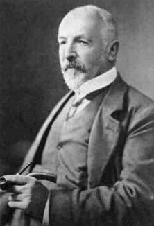
The student project Topology from Analysis begins by investigating what the question that interested Cantor means. By closely examining an example of an infinite set on which a function could be undefined but still have a unique Fourier series representation, the student is able to see why someone would write down the definition of a limit point. That same example also lays out the basic idea behind Cantor’s main result. Cantor’s definition of a derived set and its subsequent iterations are then introduced, to set up the notion that some infinite sets (e.g., point sets of finite type) are “more well-behaved" than others. Following some practice in computing derived sets, the project ends by guiding the student through Cantor’s proof of the main result of his 1872 paper. By tracing Cantor’s proof in this way, students are more naturally led to see the motivation behind the technique of proof by induction, as well as sophisticated topological concepts such as limit point and derived set.

Diagram from Cantor's 1872 proof for uniqueness of Fourier series representation,
illustrating the relationship of points on an interval in key step of his proof.
See also the author's Convergence article, “Georg Cantor at the Dawn of Point-Set Topology.”
The complete project Topology from Analysis (pdf) is ready for student use, and the LaTeX source code is available from the author by request. A set of instructor notes that explain the purpose of the project and guide the instructor through the goals of each of the individual sections is appended at the end of the student project.
This project is the sixteenth in A Series of Mini-projects from TRIUMPHS: TRansforming Instruction in Undergraduate Mathematics via Primary Historical Sources appearing in Convergence, for use in courses ranging from first-year calculus to analysis, number theory to topology, and more. Links to other mini-PSPs in the series appear below, including six additional mini-PSPs on topics in undergraduate-level analysis and topology. The full TRIUMPHS collection offers a total of six mini-PSPs and two more extensive “full-length” PSPs for use with students of topology.
Acknowledgments
The development of the student project Topology from Analysis has been partially supported by the TRansforming Instruction in Undergraduate Mathematics via Primary Historical Sources (TRIUMPHS) project with funding from the National Science Foundation’s Improving Undergraduate STEM Education Program under Grants No. 1523494, 1523561, 1523747, 1523753, 1523898, 1524065, and 1524098. Any opinions, findings, and conclusions or recommendations expressed in this project are those of the author and do not necessarily reflect the views of the National Science Foundation. The author gratefully acknowledges this support, with special thanks to TRIUMPHS PI Janet Heine Barnett, who provided assistance with the historical content of the project.
References
Cantor, G. 1871. Über trigonometrischen Reihen. Mathematische Annalen 4:139–143.
Cantor, G. 1872. Über die Ausdehnung eines Satzes aus der Theorie der trigonometrischen Reihen. Mathematische Annalen 5(1):123–132.
Scoville, N. 2012, May. Georg Cantor at the Dawn of Point-Set Topology. Convergence 9. DOI:10.4169/loci003861.
Why be so Critical? Nineteenth-Century Mathematics and the Origins of Analysis: A Mini-Primary Source Project for Introductory Analysis Students
The seventeenth century witnessed the development of calculus as the study of geometric curves in the hands of Newton, Leibniz and their immediate followers, with algebra (or 'analysis') serving as an aid to that work. This situation changed dramatically in the eighteenth century when the focus of calculus shifted instead to the study of functions, a change due largely to the influence of Euler. In the hands of Euler and his contemporaries, functions became a powerful problem solving and modelling tool in physics, astronomy, and related mathematical fields such as differential equations and the calculus of variations. Soon thereafter, mathematicians began to express concerns about calculus (analysis) and its foundations. The language, techniques and theorems that developed in response to these concerns are precisely those which students encounter in an introductory analysis course—but without the context that motivated nineteenth century analysts.
The mini-Primary Source Project (mini-PSP) presented here employs excerpts from the works of nineteenth century mathematicians as a means to introduce students to that larger context. By offering a glimpse into the problems that motivated mathematicians to shift towards a more formal and abstract study of the concepts underlying various calculus procedures and applications, the project supports students' success in making a similar shift in their own understanding of these concepts. Completing this mini-PSP early in the course can also provide students and instructors with a basis for reflection on and discussion of current standards of proof and rigor throughout the course.
|
Bernard Bolzano (1781–1848). |
Augustin-Louis Cauchy (1789–1857). |
Richard Dedekind (1831–1916). |
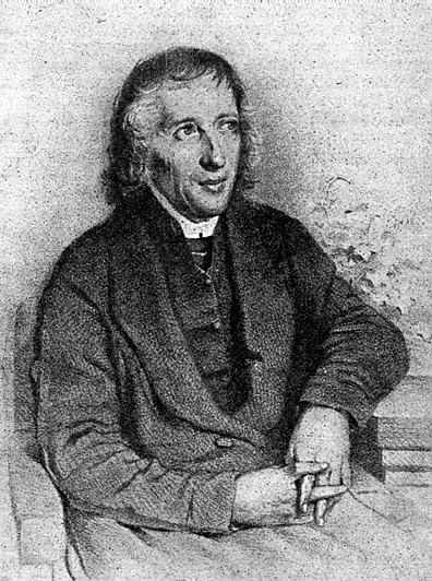
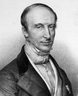

The project begins with excerpts from the writing of Bernard Bolzano [Bolzano 1817], Augustin-Louis Cauchy [Cauchy 1821; 1823] and Richard Dedekind [Dedekind 1872] in which these mathematicians described their various concerns about the state of analysis. Those concerns included, for example, a growing mistrust of geometric intuition as a valid method of proof for analytic truths. Project questions in this first section of the mini-PSP direct students' attention towards certain specific aspects of the quoted excerpts, and prompt them to compare and contrast the concerns of these three individuals.
|
In the second section of the project, students examine an extended excerpt from a letter from Niels Abel to his high school teacher, Bernt Michael Holmboe (1795–1850), written in 1826 while Abel was living in Paris. This portion of the mini-PSP again includes questions that prompt students to reflect upon the general nature of the concerns Abel expressed about the state of mathematics at the time, as well as how his concerns relate to those expressed by the authors of the earlier excerpts. Other questions in this section lead students to explore the mathematical details of examples cited by Abel as just cause for his complaints about the lack of firm foundations for power series techniques in particular.
Divergent series are on the whole devilish and it is a shame to base the slightest demonstration on them. You can get whatever you want when you use them, and they are what has produced so many failures and paradoxes. (Based on text of letter presented in [Abel 1902].) |
Niels Abel (1802–1829). |

The complete project Why be so Critical? Nineteeth-Century Mathematics and the Origins of Analysis (pdf) is ready for student use, and the LaTeX source code is available from the author by request. A set of instructor notes offering practical advice for the use of the project in the classroom is appended at the end of the student project; these include suggested Summary Discussion Notes that can be used to guide a whole class discussion of the main project themes.
This project is the second in A Series of Mini-projects from TRIUMPHS: TRansforming Instruction in Undergraduate Mathematics via Primary Historical Sources appearing in Convergence, for use in courses ranging from first year calculus to analysis, number theory to topology, and more. Links to other mini-PSPs in the series appear below. The full TRIUMPHS collection includes thirteen PSPs for use in a real analysis course.
Acknowledgments
The development of the student project Why be so Critical? Nineteeth-Century Mathematics and the Origins of Analysis has been partially supported by the TRansforming Instruction in Undergraduate Mathematics via Primary Historical Sources (TRIUMPHS) project with funding from the National Science Foundation’s Improving Undergraduate STEM Education Program under Grant No. 1523494. Any opinions, findings, and conclusions or recommendations expressed in this project are those of the author and do not necessarily reflect the views of the National Science Foundation.
References
Abel, N. 1902. Breve fra og til Abel. In Festskrift ved Hundredeaarsjubilæet for Niels Henrik Abels Fødsel, edited by E. Holst, C. Stømer and L. Sylow. Kristiana: Jacob Dybwad.
Bolzano, B. 1817. Rein analytischer Beweis des Lehrsatzes, dass zwischen je zwey Werthen, die ein entgegengesetzes Resultat gewähren, wenigstens eine reele Wurzel der Gleichung liege. Leipzig: W. Engelmann.
Cauchy, A. 1821. Cours d'Analyse de L'Ecole Royale Polytechnique. Paris: Debure.
Cauchy, A. 1823. Résumé Leçons sur le calcul infinitésimal. Paris: Debure.
Dedekind, R. 1872. Stetigkeit und irrationale Zahlen. Braunschweig: F. Vieweg und Sohn.
Wronskians and Linear Independence: A Theorem Misunderstood by Many – A Mini-Primary Source Project for Students of Differential Equations, Linear Algebra and Others
When an instructor or text presents a new mathematical idea to students, it almost always is presented in a “final form” where every statement is correct, the notation is optimized relative to current notational standards, and results logically build on previous work. Since this is all students have ever seen, they believe that is how they should be producing mathematics themselves. And when they don’t—when they make mistakes or struggle—they are understandably discouraged, since they have no reason to realize that mathematicians in fact normally struggle to arrive at their results. The pedagogical value of the mini-Primary Source Project Wronskians and Linear Independence: A Theorem Misunderstood by Many is the way it which it explicitly reveals to students the different ways in which several well-known mathematicians struggled over several decades.
The Wronskian of the functions \(f_1(x), f_2(x), \dots, f_n(x)\) is the matrix \(W\) with first row consisting of the original functions, second row consisting of their derivatives, and continuing until the \((n-1)\)st derivatives so that the matrix is square. This matrix was named for Josef-Maria Hoëné-Wronski (1776–1853), a Polish mathematician who developed certain "combinatorial sums" which ended up being the determinants of Wronskians in his Réfutation de la théorie des fonctions analytiques de Lagrange [Wronski 1812]. The following is now well known and taught in every ordinary differential equations course.
Theorem
If \(\det{(W( f_1(x), f_2(x), \dots, f_n(x)))} \neq 0\) for some \(x_0 \in I\), then \(f_1(x), f_2(x), \dots, f_n(x)\) are linearly independent on the interval \(I\).
Our students will almost universally assume the converse is true, both because many assume the converse of a true statement is always true, but also because the converse of this particular theorem absolutely seems like it should be true. Indeed, excellent mathematicians such as Charles Hermite (1822–1901), Hermann Laurent (1841–1908) and Camille Jordan (1838–1922) published (incorrect) proofs of the converse. Perhaps the above foreshadowing makes it obvious that this theorem is actually not true.
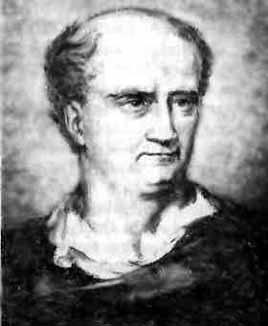

Josef-Maria Hoëné-Wronski (left) and Guiseppe Peano (right).
Convergence Portrait Gallery.
In 1889, Guiseppe Peano (1858–1932) gave counterexamples to the converse, including the one that most often appears in today’s texts [Peano 1889a, 1889b]. He also asked what conditions can be appended to the hypotheses of the converse to make it true. Various such conditions were then provided over the next 20 years, such as requiring the functions to be analytic, which often is presented in textbooks after the above Function Independence Theorem. The mini-Primary Source Project (mini-PSP) Wronskians and Linear Independence: A Theorem Misunderstood by Many tells the story of this theorem, complete with the struggles, false starts, counterexamples, and proposed corrections that went into its making. It is a concrete example of how mathematics typically progresses, and it will hopefully inspire students to be more forgiving, expecting, and accepting of their own struggles
The complete project Wronskians and Linear Independence: A Theorem Misunderstood by Many (pdf) is ready for student use, and the LaTeX source code is available from the author by request. It is designed for use in a differential equations course, a linear algebra course, or a bridge proofs course. Suggestions for each approach are included in the set of instructor notes appended to the end of the student project; these notes additionally explain the purpose of the project and guide the instructor through its goals. The interested reader is referred to the Convergence article Peano on Wronskians: A Translation (by Susannah M. Engdahl and Adam E. Parker) for more details of the story of this theorem.
This project is the eighteenth in A Series of Mini-projects from TRIUMPHS: TRansforming Instruction in Undergraduate Mathematics via Primary Historical Sources appearing in Convergence, for use in courses ranging from first-year calculus to analysis, number theory to topology, and more. Links to other mini-PSPs in the series appear below. The full TRIUMPHS collection includes an additional three PSPs for use in a differential equations course and two for use in a linear algebra course. A number of the PSPs in the collection are also suitable for use in an Introduction to Proofs course.
Acknowledgments
The development of the student project Wronskians and Linear Independence: A Theorem Misunderstood by Many has been partially supported by the TRansforming Instruction in Undergraduate Mathematics via Primary Historical Sources (TRIUMPHS) project with funding from the National Science Foundation’s Improving Undergraduate STEM Education Program under Grants No. 1523494, 1523561, 1523747, 1523753, 1523898, 1524065, and 1524098. Any opinions, findings, and conclusions or recommendations expressed in this project are those of the author and do not necessarily reflect the views of the National Science Foundation.
The author would like to thank Janet HBarnett, Danny Otero, and Dominic Klyve for inviting me to contribute to TRIUMPHS. They—along with Dave Ruch, Kenneth Monks, and David Pengelley—provided essential help in improving this mini-PSP. Additionally, Hanson Smith and his student Julia Guskind correctly pointed out that I had severely underestimated the subtlety of Task 11.
References
Engdahl, S. M., and A. E. Parker. 2011, April. Peano on Wronskians: A Translation. Convergence 8. DOI:10.4169/loci003642.
Peano, G. 1889a. Sur le déterminant Wronskien (On the Wronskian determinant). Mathesis 9:75–76.
Peano, G. 1889b. Sur les Wronskiens (On Wronskians). Mathesis 9:110–112.
Hoene-Wroński, J. M. 1812. Réfutation de la théorie des fonctions analytiques de Lagrange (Refutation of Lagrange’s theory of analytic functions). Paris: Blankenstein.