- About MAA
- Membership
- MAA Publications
- Periodicals
- Blogs
- MAA Book Series
- MAA Press (an imprint of the AMS)
- MAA Notes
- MAA Reviews
- Mathematical Communication
- Information for Libraries
- Author Resources
- Advertise with MAA
- Meetings
- Competitions
- Programs
- Communities
- MAA Sections
- SIGMAA
- MAA Connect
- Students
- MAA Awards
- Awards Booklets
- Writing Awards
- Teaching Awards
- Service Awards
- Research Awards
- Lecture Awards
- Putnam Competition Individual and Team Winners
- D. E. Shaw Group AMC 8 Awards & Certificates
- Maryam Mirzakhani AMC 10 A Awards & Certificates
- Two Sigma AMC 10 B Awards & Certificates
- Jane Street AMC 12 A Awards & Certificates
- Akamai AMC 12 B Awards & Certificates
- High School Teachers
- News
You are here
Historical Activities for Calculus - Module 2: Tangent Lines Then and Now
Module 2: Tangent Lines Then and Now
As long as mathematicians have been studying curves, they have been interested in the construction of their tangent lines. Apollonius, who lived over two thousand years ago and studied the conic curves extensively, found geometric methods for constructing tangent lines to parabolas, ellipses, and hyperbolas. In fact, Propositions 33 and 34 of Book I of Apollonius' great work, The Conics, give recipes for constructing tangents to these curves.
Apollonius' recipe for constructing tangent lines to parabolas is as follows:
Proposition I-33. Let \(P\) be a point on the parabola with vertex \(E,\) with \(PD\) perpendicular to the axis of symmetry. If \(A\) is on the axis of symmetry so that \(AE=ED,\) then \(AP\) will be tangent to the parabola at \(P.\)
Figure 11. Apollonius' recipe for constructing tangent lines to parabolas. Drag \(F,\) the focus, to change the shape of the parabola. Drag \(P,\) the point of tangency, to see the tangent line at any point on the parabola.
Apollonius' recipe for construction of tangent lines to ellipses and hyperbolas is as follows:
Proposition I-34. Let \(P\) be a point on an ellipse or hyperbola and \(PB\) the perpendicular from the point to the main axis. Let \(G\) and \(H\) be the intersections of the axis with the curve and choose \(A\) on the axis so that \[\frac{|AH|}{|AG|}=\frac{|BH|}{|BG|}.\] Then \(AP\) will be tangent to the curve at \(P.\)
Figure 12. Apollonius' recipe for construction of tangent lines to ellipses. Drag \(H\) horizontally and/or \(C\) vertically to change the shape of the ellipse. Drag \(P,\) the point of tangency, to see the tangent line at any point on the ellipse.
Figure 13. Apollonius' recipe for construction of tangent lines to hyperbolas. Drag \(H\) horizontally and/or \(C\) vertically to change the shape of the hyperbola. Drag \(P,\) the point of tangency, to see the tangent line at any point on (the right half of) the hyperbola.
Apollonius' recipes for constructing tangent lines to conic curves are easy to implement, but his methods were limited in that they could only be applied to a handful of curves. Of course, in the days of antiquity, there weren't that many curves that people were interested in studying, and so there wasn't that much of a need for a general method.
By the beginning of the seventeenth century, the collection of known curves had grown. Curves were often described as the path of a moving point; for instance, a circle can be viewed as the path traced out by a point on the outer edge of a spinning wheel. Indeed, the instruments that were used to draw curves, some of which were discussed in Module 1, underscored this notion of a curve as a path of a moving point. It was Gilles Personne de Roberval (1602-1675) who exploited this definition of a curve by viewing a tangent line as the direction in which the point is moving at a particular instant.

Figure 14. Tangent as direction of motion (click image to animate)
Consider, for example, a parabola, which, recalling Frans van Schooten’s Parabola Drawer from Module 1, can be defined as the path of point \(D\) as \(G\) moves along \(AC,\) as shown below in Figure 15.
Figure 15. Van Schooten's Parabola Drawer
As \(G\) moves along \(AC,\) the point \(D\) is being pulled simultaneously toward the point \(B\) and toward the horizontal line \(AC.\) Since \(|GD|=|BD|,\) the two forces are equal: if \(D\) moves a little toward \(B,\) it must move by the same amount toward the line \(AC\). By the parallelogram law, the direction of motion of \(D\) should be the angle bisector of \(\angle BDG.\) This angle bisector is actually the diagonal \(FH\) of the rhombus \(FGHB.\)
Both Apollonius and de Roberval used geometrical methods to construct tangent lines. One of the first algebraic methods is due to René Descartes, one of the inventors of analytic geometry. It was well known that a tangent line to a circle is always perpendicular to the radius of the circle. So Descartes' idea was to first find a circle tangent to the given curve. Then the tangent to that circle is the sought after tangent to the curve.
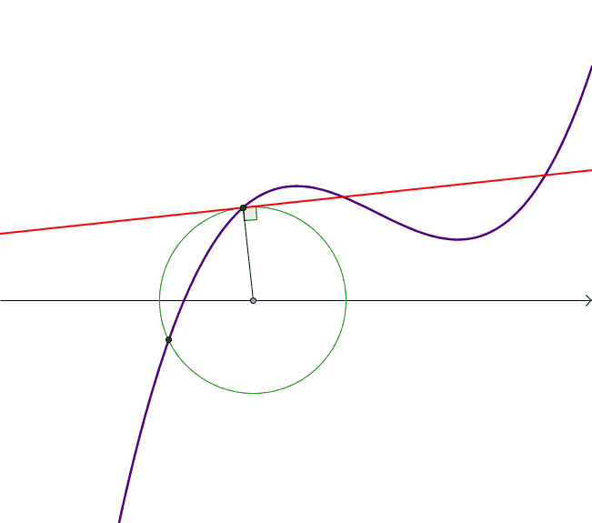
Figure 16. Descartes' Method: Tangent to curve is perpendicular to radius of tangent circle. (Click image to animate.)
It was Pierre de Fermat who came up with essentially the method used today to construct tangent lines, by viewing the tangent as the limit of secant lines through the given point \(A\) and a nearby point \(B\) on the curve, where \(B\) approaches and eventually becomes \(A.\)

Figure 17. Fermat's method of constructing tangent lines (click image to animate)
Fermat's method, although it worked in practice, was not without controversy. If \(A=(a,f(a))\) is a point on the curve \(y=f(x),\) and \(B=(a+e,f(a+e))\) is a nearby point, the slope of the line \(AB\) is perfectly well-defined as long as \(A\) and \(B\) are distinct, i.e. \(e\neq 0\), but how do we define the slope when \(e=0\) so that \(B=A?\) This seeming inconsistency invited much criticism, the most famous coming from the Irish philosopher and bishop, George Berkeley (1685-1753), in a pamphlet he published in 1734 called The Analyst. Here Bishop Berkeley ridiculed the increments \(e,\) calling them the “ghosts of departed quantities." In fact, Descartes developed his method discussed above as a way to get around these difficulties. You can see below how, as \(B\) approaches \(A,\) the circle with center \(O\) on the \(x\)-axis that goes through \(A\) and \(B\) is well-defined, even when \(A=B.\) However the line through \(A\) and \(B\) cannot be well-defined when \(A=B.\)

Figure 18. Descartes' method compared to Fermat's method (click image to animate)
Unfortunately, Descartes' method did not work very well except for some simple curves, because of the burdensome algebra involved in finding the unique circle with center on the \(x\)-axis that intersects the curve only once at \(A.\)
In spite of the problems with the logical foundations of the subject, nobody could dispute that the techniques worked. And so Fermat is credited with the invention of the differential calculus since he developed this method in 1629 and used it successfully to compute subtangents of a large collection of curves. It wasn't until the nineteenth century that the controversies and problems were satisfactorily addressed by the French mathematician Augustin-Louis Cauchy (1789-1857), who gave a precise definition of derivative in terms of a new concept called limit. This led to the definition that we use today.
Exercises
Figure 19. This applet for Exercise 5 implements recipes of Apollonius to construct tangent lines to parabolas, ellipses, and hyperbolas.
Exercise 5.
Use the recipes prescribed by Apollonius and the applet in Figure 19, above, to construct the following tangent lines.
(a) The tangent line to the parabola \(y=\frac{x^2}{4}+1\) at the point \((4,5).\)
(b) The tangent line to the ellipse \(\frac{x^2}{25}+\frac{y^2}{9}=1\) at the point \((3,2.4).\)
(c) The tangent line to the hyperbola \(\frac{x^2}{16}-\frac{y^2}{9}=1\) at the point \((5,2.25).\)
Exercise 6.
In this exercise you will use de Roberval's method to construct tangent lines to several curves.
Figure 20. This applet for Exercise 6, part a, illustrates the standard construction of the parabola using focus \(F\) and directrix \(OB\).
(a) The applet in Figure 20, above, illustrates the construction of the parabola as the locus of points \(P\) that are equidistant from a fixed point \(F\) (the focus) and a fixed line \(OB\) (the directrix). You can see that as you drag the point \(B,\) the distances \(BP\) and \(PF\) are always equal.
There are two forces acting on \(P\): one toward \(F\) and one toward the horizontal line \(OB.\) Since \(|FP|=|BP|,\) the two forces are equal, meaning if \(P\) moves a little toward \(F,\) it must move by the same amount toward the line. Hence the direction of motion, by the parallelogram law, should be the angle bisector of \(\angle FPB.\) Construct the angle bisector to verify that this does indeed appear to be tangent to the curve at every point of the parabola. To do this:
Click on the angle bisector tool in the toolbar, then on the segment \(FP,\) and then on the segment \(PB.\) You'll get two lines, perpendicular to each other. Click the Move tool, then right-click on the line you don't want and select Show Object to hide it. You can drag \(B\) to verify that this construction works for every point on the parabola.
Figure 21. This applet for Exercise 6, part b, illustrates the standard construction of the ellipse using two foci \(F_1\) and \(F_2.\)
(b) The applet in Figure 21, above, illustrates the construction of the ellipse as the locus of points \(P\) such that the sum of \(P\)'s distances from two fixed points \(F_1\) and \(F_2\) is constant. Note that as you drag the point \(P,\) the sum \(|PF_1|+|PF_2|\) remains constant.
Since \(|PF_1|+|PF_2|\) is constant, each time \(P\) moves toward \(F_1\) it must move the same distance away from \(F_2.\) So there are two equal forces acting on \(P,\) one toward one of the foci, the second away from the other focus. So again you can construct the tangent line as an angle bisector. Construct the tangent to the ellipse at any point \(P.\) Make sure your construction works at every point of the ellipse.
Figure 22. This applet for Exercise 6, part c, illustrates the standard construction of the hyperbola using two foci \(F_1\) and \(F_2.\)
(c) The applet in Figure 22, above, is the construction of the hyperbola as the locus of points \(P\) such that the difference of \(P\)'s distances from two fixed points \(F_1\) and \(F_2\) is constant. Note that as you drag the point \(P,\) the difference \(|PF_1-PF_2|\) remains constant. Construct the tangent to the hyperbola at any point \(P.\) Make sure your construction works at every point of the hyperbola.
Figure 23. This applet for Exercise 6, part d, illustrates the cycloid as the path traced by a point on the circumference of a circle rolling along a horizontal line.
(d) The cycloid, illustrated in Figure 23, above, played a very important part in the history of the calculus, and its properties were studied extensively during the sixteenth and seventeenth centuries. It is the path traced out by a point on the circumference of a circle as the circle rolls on a horizontal line. Use de Roberval's method to construct the tangent line at any point \(P\) of the cycloid.
Figure 24. This applet for Exercise 6, part e, illustrates the epicycloid as the path traced by a point on the circumference of one circle rolling along the outside of another circle.
(e) The epicycloid, illustrated in Figure 24, above, is the path traced out by a point on the circumference of a circle as the circle rolls on the outside of another circle. Use de Roberval's method to construct the tangent line at any point \(P\) of the cycloid.
Exercise 7.
In this exercise, you will use Descartes' method to find tangent lines to the curve \(y=\sqrt{4x}.\) The method consists of first finding a circle tangent to the curve. Then the tangent line to the curve will be the same as the tangent line to the circle, which is easily constructed since it is perpendicular to the radius.
Figure 25. Applet for Exercise 7
(a) The applet shown above in Figure 25 contains: a graph of \(y=\sqrt{4x},\) the point \(A=(1,2)\) which is on this curve, a point \(O\) on the \(x\)-axis, and a circle with center \(O\) and radius \(OA.\) In general, depending on where point \(O\) is, this circle will cross the curve at two points \(A\) and \(B.\) Now drag \(O\) along the \(x\)-axis until the two points of intersection \(A\) and \(B\) merge into one. The resulting circle touches the curve at a single point and so is tangent to the curve. Now you can compute the slope of the tangent, since it is perpendicular to \(OA.\) Type the equation of the tangent line into the purple input box to graph it and verify that it is indeed tangent to \(y=\sqrt{4x}\) at \(A=(1,2).\)
(b) Repeat with \(A=(9,6)\) and enter the equation of the tangent line into the blue input box.
References
J. L. Coolidge, The Story of Tangents, The American Mathematical Monthly, Vol. 58, No. 7. (1951), pp. 449-462.
Paul R. Wolfson, The Crooked Made Straight: Roberval and Newton on Tangents, The American Mathematical Monthly, Vol. 108, No. 3 (2001), pp. 206-216.
Gabriela R. Sanchis (Elizabethtown College), "Historical Activities for Calculus - Module 2: Tangent Lines Then and Now," Convergence (June 2014)


