Math Origins: The Language of Change

As originally conceived, this series of articles was meant to explore the often-labyrinthine process by which notations in the undergraduate mathematical curriculum came about. Over the course of the past five articles, it has become something more than that: a testament to tumult and confusion, and to the complexity of that very human endeavor of mathematical inquiry.

Thus far in the Math Origins series, we have explored number theory in The Totient Function, asymptotic notations in Orders of Growth, linear algebra in Eigenvectors and Eigenvalues, and mathematical logic in The Logical Ideas and The Logical Symbols. In each of these articles, the original meaning of a symbol or concept has evolved through the centuries before landing in today’s undergraduate textbooks. My hope is that seeing the explicit changes in both symbols and concepts illuminates our own role in the ongoing story of mathematics—as the readers and writers of the present, we have the power to build upon and modify the concepts of the past. It is fitting, then, that this series end with a reflection on the mathematics of change: those symbols from differential calculus that are often a student’s first exposure to a deeper, more creative mathematics. We will see, as we have in each article of the series, that many competing notations were proposed and used, and that no true consensus was reached—even today, many ways of representing mathematical change coexist (however tenuously) in textbooks and classrooms around the world.

The Early History of Calculus

We will not give a substantial history of Calculus here, since that subject has been examined in great detail elsewhere. (For a general narrative on history of the derivative concept, see [Gra]. The review by [Hun] of [Son] suggests readings on the infamous Newton-Leibniz priority dispute.) Here, we first look to the notations that emerged in the late 17th century, primarily due to Isaac Newton and Gottfried Wilhelm von Leibniz. According to Cajori, Newton used his ‘overdot’ notation as early as 1665 [Caj, p. 197], though I have been unable to find direct evidence of it. It does not appear in his initial work on the Calculus, "De Analysi per aequationes numero terminorum infinitas," which Newton had written by 1669 [New1]. However, this notation does appear in the De Methodis Serierum et Fluxionum (later published in English as The Method of Fluxions and Infinite Series), which had been written by 1671 even though it did not appear in print until 1736, fully 19 years after Newton's death.

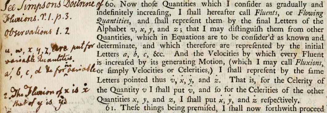
Figure 1. Newton's definitions for fluents and fluxions in The Method of Fluxions and Infinite Series [New2, p. 20] (pub. 1736), with John Adams’s handwritten notes in the margin. This particular volume is in the John Adams Library at the Boston Public Library. Image courtesy of Archive.org.

In Figure 1, we see a fully-formed theory of fluents and fluxions, Newton’s way of describing variable quantities and their instantaneous rates of change. Interestingly, this image [New2, p. 20] includes margin notes by John Adams, who apparently read this text in combination with Thomas Simpson’s 1737 book, Doctrine and Application of Fluxions [Sim], some pages of which feature as a Convergence Mathematical Treasure. Following Adams’s cryptic margin note, we find an equivalent definition of fluxions from Simpson on page 3 of Part I of the Doctrine and Application of Fluxions. By this time, Newton’s notation predominated in Britain, and Simpson’s work is no exception. Simpson’s first example of the utility of Newton’s notation is the calculation of the fluxion of x².

Figure 2. In his Doctrine and Application of Fluxions [Sim, p. 3], (pub. 1737), Thomas Simpson used a typical combination of geometric and analytic exposition to find the fluxion for x². Image courtesy of HathiTrust Digital Library.

Significantly, we see here how geometric the mathematical sciences still were; this preference for geometric arguments as the true justification for mathematical truths would continue well into the 19th century. So, too, would Newton's fluxional notation—English mathematician John Wallis adopted the notation in his 1693 text, De algebra tractatus [Wal], and extended it to include higher-order derivatives.

Figure 3. John Wallis's extension of Newton's ‘overdot’ notation to higher-order fluxions, from De algebra tractatus [Wal, p. 392] (pub. 1693). Image courtesy of HathiTrust Digital Library.

Here we see a proliferation of dots, denoting second-order, third-order, and even fourth-order derivatives! It should be noted that Newton himself used this extended notation in Tractatus de quadratura curvarum (pub. 1704), which he wrote in the same year that Wallis’s De algebra tractatus was printed.

At the same time that these geometers were developing the fluxional calculus in Britain, Leibniz and his disciples were exploring the same notational questions for their differential calculus. Returning to Cajori [Caj, p. 204], we find that Leibniz used a lower-case d for the differential as early as 1675, though it did not appear in print until 1684. That year, his “Nova methodus pro maximis et minimis” (“New method for finding maxima and minima”) was published in the Acta Eruditorum [Lei]. In it, Leibniz presented a method of calculating the tangents to a curve, including rules that would be familiar to any student of Calculus today: differentiating constant multiples, sums and differences, products, quotients and powers. Of course, Leibniz did not employ the now-common analytic geometry of functions and coordinates, instead using a geometric approach reminiscent of René Descartes’ La Géometrie. For a given point on a curve, Leibniz determined the length of a tangent line segment from the ratio of the point's “ordinate” to its “abscissa.” (In more modern language, we would say that Leibniz’s abscissa is a distance measured along the vertical coordinate axis, and the ordinate is the length of the perpendicular connecting the curve to the vertical coordinate axis.)

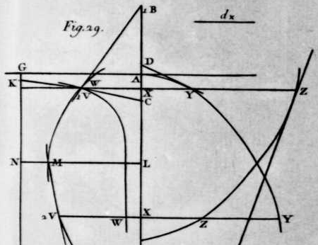
Figure 4. The geometric problem from Leibniz’s “Nova methodus pro maximis et minimis” [Lei] (pub. 1684), as it was reprinted in his collected works. Image courtesy of HathiTrust Digital Library.

While Leibniz used four curves to explain his method, we focus on one—the curve YYA in Figure 4. For this early version of the characteristic triangle, Leibniz constructed the line YD tangent to YYA, taking the ratio dy:dx = YX:YD to define the differential of y (the process was similar for the other variables v, w, z). Thereafter, he used an overline (also known as a vinculum) to denote the quantity whose differential he wished to find. Here is how some typical differentiation rules appeared in this notation:

• the constant multiple rule \(d\overline{ax} = a dx\),

• an addition and subtraction rule \(d\overline{z-y+w+x} = dz-dy+dw+dx\),

• the multiplication rule \(d\overline{xv} = x\,dv+v\,dx\).

In fact, Leibniz went as far as calculating second-order differentials—in his words, the “differences of the differences”—using the double-d notation (e.g., ddv). This notation is limited by Leibniz’s conception of the geometric quantities involved, but his new method for tangents was given a clear and consistent notation from the beginning.

Differences of Differences

As the decades passed, Newton’s fluxional Calculus held sway in Britain, while Leibniz’s differential predominated in continental Europe. One of the most prominent inheritors of the differential was Johann Bernoulli, the Swiss-born brother of Jakob and the mind behind the Marquis de L'Hôpital’s Analyse Infinitments Petits (pub. 1696), the first printed Calculus textbook. Here, we look at an excerpt from his 1694 article, "Effectionis omnium quadraturarum & rectificationum curvarum per seriem quandam generalissimam" [Ber1]. Following Leibniz’s use of d for differences and dd for “differences of the differences,” Bernoulli used the notations ddd and dddd in his derivation of a power series for \(x = b^{y/a}-a\).

Figure 5. Johann Bernoulli used multiple d’s to denote higher-order differentials in the power series for \(x = b^{y/a}-a\), in the 1694 paper, “Effectionis omnium quadraturarum & rectificationum curvarum per seriem quandam generalissimam” [Ber1, pp. 126-127]. Image courtesy of Google Books.

Parsing Bernoulli’s analysis, we see that he began with the ratio \(dy = a dx : r\), equivalent to \(\frac{dy}{dx} = \frac{a}{r}\), and used successive differentiation to obtain a series representation for y. In fact, Bernoulli did more than this—he used r = a+x, and while he did not evaluate the integral of dy, we know that \(y=a\cdot \ln(a+x)\) is an antiderivative. So in today's terminology, Bernoulli’s series representation is a Taylor series representation of a logarithm function. Taking a wider view, we can see here how the differential has now grown to include purely analytic methods, without direct consideration of curves and tangents.

At roughly the same time Bernoulli was writing the "Effectionis," he and Leibniz were corresponding with each other on the Calculus, and it is here that we get some clarity on their notational methods. In 1698, Leibniz wrote to Bernoulli suggesting that, when z is a function of x, the ratio of differences dz/dx be denoted with a ‘broken d’ notation—a dz with a horizontal line struck through the d, as we see below [Per, p. 526].

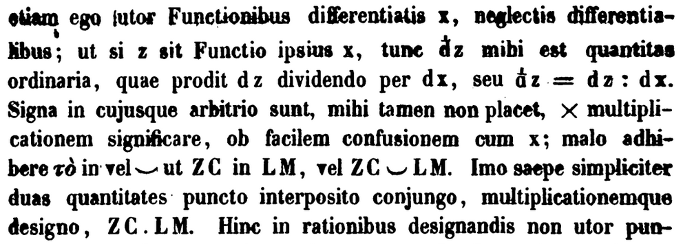
Figure 6. In a 1698 letter to Johann Bernoulli, Leibniz described his use of a ‘broken d’ notation for the difference ratio dz/dx. Image courtesy of HathiTrust Digital Library.

Perhaps the horizontal line was meant to evoke a fraction. At any rate, Bernoulli responded enthusiastically [Per, p. 531]:

Figure 7. Bernoulli’s response to Leibniz’s ‘broken d’ notation for denoting a ratio of differences (1698), indicating that he had used D for this purpose. Image courtesy of HathiTrust Digital Library.

Even though Bernoulli expressed his preference for Leibniz’s notation, the broken dz has not persisted. According to Cajori [Caj, p. 182], Leibniz never used the broken d in his published work, providing “a fine example of masterful self-control.” As we will see, it is Bernoulli’s capital D that persists in many of today's Calculus textbooks.

Delta, Del, and Nabla

As any student of multivariable Calculus knows, the letter d is not the end of this story. Today, the symbols \(\Delta\) and \(\nabla\) are often used to describe the theory of differentials in a higher-dimensional setting. Additionally, the Greek \(\Delta\) (capital delta) is known to students of pre-Calculus and physics as another way to represent change in a quantity. My own experience with \(\Delta\) as a student was that it denoted discrete (that is, not infinitesimal) differences: so \(\Delta y/\Delta x\) would represent the change in \(y\) with respect to \(x\) over a fixed interval, while \(dy/dx\) would represent the change in \(y\) with respect to \(x\) at an instant. However, the earliest uses of \(\Delta\) were less precise. For example, Johann Bernoulli published a solution to an isoperimetric problem in 1706 (originally posed by Bernoulli himself in 1697) in which he made use of \(\Delta\) to describe a continuous change.

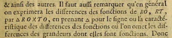
Figure 8. Johann Bernoulli's use of \(\Delta\) in his solution to an isoperimetric problem, published in the Paris Mémoires for 1706 [Ber2]. Image courtesy of Biodiversity Heritage Library.

Roughly translated, Bernoulli used \(\Delta\) to denote the “symbol for the differences of the functions where one omits the differences of the magnitudes of which they are functions.” Nearly 200 years later, the Swedish mathematician and historian Gustaf Eneström [Ene, p. 21] explained Bernoulli’s cumbersome language in this way:

\(\Delta RO\) is not the difference of RO, but the difference of a certain function of RO; moreover, we find easily that here, the word "difference" does not refer to a finite difference, but corresponds to the modern term "derivative," and consequently, the symbol \(\Delta\) must be defined not by the equation \(\Delta f(x) = f(x+h)-f(x)\), where \(f(x)\) is an arbitrary function, but by the equation \(\Delta x = \frac{df(x)}{dx}\), where \(f(x)\) is a function known in advance.

So, at this early stage, \(\Delta\) was a generalized differential that applied to a function of x. Also, the perceptive reader might notice the appearance of the word function in Bernoulli’s paper. While the notation for it came later, we see here an intuitive use of the word for any quantity that is dependent on another.

Through the 18th century, writers from Leonhard Euler to Maria Agnesi to Joseph-Louis Lagrange employed versions of the lower-case d for differentials in their work on Calculus. However, the usage of this notation had changed considerably from Leibniz’s day. One of the more underrated notational changes came from Alexis Fontaine, who wrote a manuscript in 1738 in which he introduced the familiar “fraction form” for ratios of differences, which allowed for the writer to express partial derivatives more clearly. While this manuscript was not published until 1764, knowledge of Fontaine’s contributions circulated widely during this time, eventually being adopted by most mathematicians of the day. One early mention of the fraction notation was in a 1740 letter by Alexis Clairaut to Euler [OO, pp. 68-69]:

Mr. Fontaine states the general method: \(\mu\) being an arbitrary function of \(x\) and \(y\), the difference of \(\int\mu\,dx\) in varying \(y\) and keeping \(x\) constant is \(dy \int\frac{d\mu}{dy} dx\); we mean by \(\frac{d\mu}{dy}\) the quantity which we obtain from differentiating \(\mu\), with variable \(y\) and \(x\) remaining constant...

Clairaut went on to explain how this notation unlocked the possibility of representing partial derivatives for functions of several variables. When Fontaine’s manuscript was printed 24 years later in the Paris Mémoires, we can see he made this exact point in “Le Calcul Intégral.”

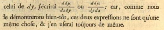
Figure 9. Fontaine's notation for differentials in "Le Calcul Intégral," a widely-read manuscript written in 1738 and only printed in 1764. Image courtesy of Google Books.

Identifying \(\mu\) as a function of variables \(p\), \(x\), \(y\), \(z\), etc., Fontaine described \(\frac{d\mu}{dx}\) as “the coefficient of \(dx\) in the differential of \(\mu\),” which is essentially the same as a partial derivative. We can see here that he went on to apply his notation to higher-order partial derivatives, even going as far to note the equality of the mixed partials \(\frac{dd\mu}{dx dy}\) and \(\frac{dd\mu}{dy dx}\).

A modern reader will notice the absence of the symbol \(\partial\) in Fontaine's notation. Indeed, this symbol seems to find its origin in a 1786 paper by Adrien-Marie Legendre [Leg]. In his “Mémoire sur la manière de distinguer les maxima des minima dans le Calcul des Variations” (“Memoir on the method for distinguishing maxima and minima in the Calculus of Variations”), Legendre used the Greek \(\delta\) to represent the total differential, with the variant \(\partial\) representing partial derivatives in the calculation.

Figure 10. In the 1786 paper, “Mémoire sur la manière de distinguer les maxima des minima dans le Calcul des Variations” [Leg], Legendre modified Fontaine's notation, using \(\partial\) and \(\delta\) for partial differentials. Image courtesy of the Bibliothèque Nationale de France's Gallica collection.

In a footnote marked with a (*) in the image above, Legendre explained his use of this symbol:

To avoid any ambiguity, I will represent by \(\frac{\partial v}{\partial x}\) the coefficient of dx in the differential of v, and by \(\frac{dv}{dx}\) the complete differential of v divided by dx.

So we see that, by the close of the 18th century, the notation for differentials had expanded to include multivariate functions, with notions of total and partial differentials having their own symbols. What began with Leibniz's simple dx in the "Nova methodus pro maximis et minimis" now included D, \(\Delta\), \(\partial\), \(\delta\), each with their varying contexts.

Diverging Derivatives

As Calculus advanced into the 19th century, many new developments expanded the notion of “change” in the minds of mathematicians. In particular, this included the incorporation of the vector concept into Calculus, providing many new ways of defining differentials for more sophisticated situations. To close out this article (and this series), we take a brief tour of the various differential notations that have appeared in multivariate Calculus in the past two centuries.

We have already seen that, as early as 1706, Johann Bernoulli used the Greek letter \(\Delta\) to denote the derivative for a single-variable function. However, many students of vector Calculus know this symbol as the cousin of \(\nabla\)—variously called del or nabla—used to denote the divergence of a vector field. Specifically, for a vector field \(\vec{F} = \langle F_x, F_y, F_z\rangle\), the divergence may be denoted by \(\nabla\cdot\vec{F}\), which is to say that the operator \(\nabla=\langle\frac{\partial}{\partial x}, \frac{\partial}{\partial y}, \frac{\partial}{\partial z}\rangle\) is combined with \(\vec{F}\) using a formal inner product. Informally, the divergence measures the extent to which the vector field “pushes” out of a given region. Since our interest lies in the symbols used to represent this concept, it is worth noting that the inverted \(\Delta\) was not the only way this concept has been expressed. William Rowan Hamilton used a sideways \(\Delta\) in his paper, “On the Expression and Proof of Paschal’s Theorem by Means of Quaternions” [Ham] which appeared in the Royal Irish Academy's Proceedings for the years 1845–1847. Here is Hamilton's original definition from page 291, written from the perspective of the Academy:

the following more general characteristic of operation,

\(i\frac{\text{d}}{\text{d}x}+j\frac{\text{d}}{\text{d}x}+k\frac{\text{d}}{\text{d}x} = {\Large \triangleleft}\),

in which \(x\), \(y\), \(z\) are the ordinary rectangular coordinates, while \(i\), \(j\), \(k\) are his own coordinate imaginary units, appears to him to be one of great importance in many researches. This will be felt (he thinks) as soon as it is perceived that with this meaning of \({\Large \triangleleft}\) the equation

\(\left(\frac{\text{d}}{\text{d}x}\right)^2+\left(\frac{\text{d}}{\text{d}y}\right)^2+\left(\frac{\text{d}}{\text{d}z}\right)^2 = -{\Large \triangleleft}^2\),

is satisfied in virtue of the fundamental relations between his symbols \(i\), \(j\), \(k\).

A version of Hamilton's notation was adopted by Peter Tait in his 1867 text, An Elementary Treatise on Quaternions, though by that time the \(\Delta\) symbol had completed its rotation to become \(\nabla\). Beginning on p. 221, Tait carried out a nearly-identical calculation to that of Hamilton, applying the operator \(\nabla\) to a vector field for the first time:

Figure 11. Peter Tait inverted \(\Delta\) to use \(\nabla\) in An Elementary Treatise on Quaternions [Tai, p. 221] (pub. 1867). Image courtesy of Archive.org.

We see the \(\nabla\) symbol is first used to denote Hamilton’s differential operator, and then repeated to produce the now-named Laplace operator \(\nabla^2\). As to the symbol itself, it is sometimes named as “del” or “nabla,” with the former being an abbreviation of the word “delta.” The latter was suggested to Tait by the biblical scholar and encyclopedist William Robertson Smith, who was inspired by the Greek \(\nu\alpha\beta\lambda\alpha\), meaning “harp,” since he considered the inverted \(\Delta\) to resemble a harp.

As with all good origin stories, the picture becomes blurred as time passes. By the late 19th century, many different symbols were in use across the world, and while some early symbol choices (like Leibniz’s “broken d”) were rejected, many others had their acolytes. Many in Britain, including many physicists, continued to use Newton’s overdot notation—and many still do! Others use Leibniz’s d for single-variable Calculus, but adopt \(\partial\) and \(\nabla\) when in a multivariable setting. And while the capital letter \(\Delta\) is often reserved for discrete differences, this rule is not always strictly observed.

As to the capital D, it achieved a minor renaissance in the United States due to a historical accident. Before the 19th century, the Calculus done in the British colonies was heavily Newtonian (as suggested by Adams’ reliance on Newton’s fluxions in his studies). This began to change in the early 19th century. In particular, the American mathematician Benjamin Peirce adopted the capital D as his primary notation for the derivative in his 1841 text, Curves, Functions, and Forces. Peirce, a long-serving Harvard professor and an influential mathematical figure in the early years of the United States, saw his notation adopted at schools across the country. While the capital D no longer retains the central role in American classrooms that it once did, it does show that sometimes a notational choice is more of an accident than a true choice.

References

[Ber1] Bernoulli, Johann. "Effectionis omnium quadraturarum & rectificationum curvarum per seriem quandam generalissimam." Johannis Bernoulli Opera Omnia, Vol. 1, pp. 125–128. Lausanne and Geneva, 1742.

[Ber2] Bernoulli, Johann. "Du Problême proposé par M. Jacques Bernoulli dans les Actes de Leipsik du mois de May de l'année 1697." Mémoires de à l'Académie Royale des Sciences, année 1706 (1731), 235–245.

[Caj] Cajori, Florian. A History of Mathematical Notations. Vol. 2. Chicago: Open Court Publishing Co., 1928.

[Ene] Eneström, Gustaf. "Recensionen – Analyses." Bibliotheca Mathematica, Series 2, 10 (1896), 17–26.

[Fon] Fontaine, Alexis. "Le Calcul Intégral." Mémoires donnés à l'Académie Royale des Sciences, non imprimés dans leur temps (1764), 24–28.

[Gra] Grabiner, Judith. "The Changing Concept of Change: The Derivative from Fermat to Weierstrass." Math. Magazine 56 (no. 4) (1983), 295–206.

[Ham] Hamilton, William Rowan. "On the Expression and Proof of Paschal's Theorem by Means of Quaternions." Proceedings of the Royal Irish Academy (1836–1869) 3 (1844–1847), 273–294.

[Hun] Hunachek, Mark. Review of The History of the Priority Dispute between Newton and Leibniz, by Thomas Sonar. MAA Reviews, 12 June 2018.

[Leg] Legendre, Adrien-Marie. "Mémoire sur la manière de distinguer les maxima des minima dans le Calcul des Variations." Mémoires de à l'Académie Royale des Sciences (1786), 7–37.

[Lei] Leibniz, Gottfried. "Nova Methodus Pro Maximis et Minimis, itemque tangentibus, que nec fractas, nec irrationales quantitates moratur, et singulare pro illis calculi genus." Acta Eruditorum (1684), 467–473.

[New1] Newton, Isaac. De Analysi per aequationes numero terminorum infinitas. Letter to John Collins, 31 July 1669. Published in London: William Pearson, 1711.

[New2] Newton, Isaac. The Method of Fluxions and Infinite Series. London: Henry Woodfall, 1736.

[OO] Lemmermeyer, F. and M. Mattmuller, eds. Leonhard Euler Opera Omnia: Series Quarta A. Volume 5: Commercium Epistolicum. Basel: Springer, 1980.

[Per] Pertz, Georg H., ed. Leibnizens gesammelte Werke. Vol. 3. Halle: H. W. Schmidt, 1856.

[Sim] Simpson, Thomas. The Doctrine and Application of Fluxions. London: Knight and Compton, 1737.

[Son] Sonar, Thomas. The History of the Priority Dispute between Newton and Leibniz. Birkhäuser, 2018.

[Tai] Tait, Peter. An Elementary Treatise on Quaternions. Oxford: Clarendon Press, 1867.

[Wal] Wallis, John. De algebra tractatus. Oxford, 1693.