- About MAA
- Membership
- MAA Publications
- Periodicals
- Blogs
- MAA Book Series
- MAA Press (an imprint of the AMS)
- MAA Notes
- MAA Reviews
- Mathematical Communication
- Information for Libraries
- Author Resources
- Advertise with MAA
- Meetings
- Competitions
- Programs
- Communities
- MAA Sections
- SIGMAA
- MAA Connect
- Students
- MAA Awards
- Awards Booklets
- Writing Awards
- Teaching Awards
- Service Awards
- Research Awards
- Lecture Awards
- Putnam Competition Individual and Team Winners
- D. E. Shaw Group AMC 8 Awards & Certificates
- Maryam Mirzakhani AMC 10 A Awards & Certificates
- Two Sigma AMC 10 B Awards & Certificates
- Jane Street AMC 12 A Awards & Certificates
- Akamai AMC 12 B Awards & Certificates
- High School Teachers
- News
You are here
Servois' 1817 "Memoir on Quadratures" – Student Exercises on The Trapezoidal Rule and Kramp's Algorithm
In this section and the next, we provide suggestions for student exercises related to Servois' memoir on numerical integration. We begin with some additional detail about Kramp's notation and algorithm which forms the basis of the exercises at the end of this section.
The Composite Trapezoidal Rule (or just the Trapezoidal Rule) gives an approximate value of a definite integral
\[ \int^b_a f(x) \, dx. \]
To apply the rule, we let \(\Delta x = \frac{b-a}{n}\) and define \(x_i = a + k\Delta x\) for \(0 \le i \le n\). Then
\[ \frac{\Delta x}{2}\left[f(x_0) +2 f(x_1) + 2 f(x_2) + \cdots + 2 f(x_{n-1}) + f(x_n)\right] \,\,\,\,\,\,\,\mbox{(XI)}\]
provides an approximate value of the definite integral, with better and better approximations as the value of \(n\) increases.
In his article [Kramp 1815a], Christian Kramp presented an algorithm that takes a few such approximate values of a definite integral, for different small values of \(n\), and uses an extrapolation procedure to produce a new estimate that is much more accurate than those given by the Trapezoidal Rule.
Let's illustrate Kramp's algorithm by applying it to the definite integral
\[ \int_1^2 \frac{1}{x} dx. \]
Kramp chose this example because we can compare the approximations to the exact value of the integral, which is \(\ln 2 = 0.69314718\cdots\).
The first approximation comes from taking \(n=1\). This gives
\[ S_4 = \frac{1}{2} \left[f(1)+f(2)\right] = \frac{3}{4} = 0.75. \]
The second approximation is given by \(n=2\):
\[ S_2 = \frac{\frac{1}{2}}{2} \left[f(1)+ 2f\left(\frac{3}{2}\right) + f(2)\right] = \frac{17}{24} = 0.708\overline{3}. \]
We take one more approximation, this time with \(n=4\):
\[ S_1 = \frac{\frac{1}{4}}{2} \left[f(1)+ 2f\left(\frac{5}{4}\right)+ 2f\left(\frac{3}{2}\right)+ 2f\left(\frac{7}{4}\right) + f(2)\right] = \frac{1171}{1680} \approx 0.697023810. \]
Let's pause to make some comments about the subscripts, which seem to be wrong. The first observation is that Kramp actually used this notation. In the 1810s some mathematicians used subscripts, which were then a recent invention, but many others did not. Nowhere in his “Memoir on Quadratures” [Servois 1817], nor in any of his other works, did Servois make use of subscripts. None of the great mathematicians of the 17th and 18th centuries had access to this useful notational device.
As for the case in point, Kramp took the smallest value of \(\Delta x = \frac{1}{4}\) as a sort of unit for all of the approximations. Let's call it \(\omega\). Then the first approximation above, with \(n=1\), comes from taking \(\Delta x = 4 \omega\), and so he denoted it \(S_4\). The second approximation has \(\Delta x = 2 \omega\), so it is called \(S_2\). Finally, the last and most accurate estimate uses \(\Delta x = 1 \omega\), so it is called \(S_1\). The larger \(n\) is, the smaller \(\Delta x\) is and the more accurate the approximation is. So intuitively, the value of \(S_0\), which may be thought of as a limit as \(\Delta x\) goes to zero, should be the value of the integral. The problem then is to use \(S_4\), \(S_2\) and \(S_1\) to estimate \(S_0\).
We let \(S(x)\) be the function that gives the values of \(S_n\) (Kramp used \(F\) for this function). Kramp assumed that the function \(S\) was an even function, although he didn't explain why, other than to say that he wanted \(S'(0)=0\). Therefore the MacLaurin series for \(S\) is
\[ S(x) = A + Bx^2 + Cx^4 + D x^6 + \cdots .\]
We then expect that \(S(0)=A\) should be the value of the definite integral, or at least a good estimate to it.
In the current example, we only have three estimates, so we can only get the approximate values of the first three coefficients of the the MacLaurin series. In other words, we'll fit our three data points to the equation
\[ S_n = A + Bn^2 +Cn^4. \]
This gives a \(3\times 3\) linear system:
\[\begin{array}{llrlrll} A & + & B & + & C & = & \frac{1171}{1680} \\ A & + & 4B & + & 16 C & = & \frac{17}{24} \\ A & + & 16B & + & 256C & = & \frac{3}{4} \end{array} \]
This system is small enough to solve by hand. The solution gives the value
\[ A = \frac{4367}{6300} \approx 0.693174603, \]
which is very close to \(\ln 2\). The absolute error of the approximation is \(|A - \ln 2| \approx 0.0000274\), which is less than .004% of the actual value of the integral. This compares with an absolute error of about \(0.00388\) in the estimate \(S_4\), more than 100 times bigger.
Kramp's Algorithm
Let \(N\) be a natural number, preferably a composite number with many factors. Let \(m = \sigma(N)\), the number of factors of \(N\). We estimate the integral
\[ I = \int^b_a f(x) \, dx \]
by \(m\) different applications of the Trapezoidal Rule. Let \(\omega = \frac{b-a}{N}\).
Now for each factor \(n\) of \(N\), let \(k=\frac{N}{n}\) and let \(S_k\) be the Trapezoidal Rule approximation of the integral \(I\) with \(\Delta x = k \omega\) given by formula (XI).
Suppose that
\[ S(x) = A_0 + A_1 x^2 + \cdots A_m x^{2(m-1)} \]
and fit the values of \(S_k\) to this equation. This gives an \(m \times m\) linear system
\[\begin{array}{llrllrlcl} A_0 & + & A_1 & + & \cdots & + & A_m & = & S_1\\ A_0 & + & 2A_1 & + & \cdots & + & 2^{2(m-1)} A_m & = & S_2\\ &\vdots&&\vdots&&\vdots&&\vdots \\ A_0 & + & kA_1 & + & \cdots & + & k^{2(m-1)} A_m & = & S_k\\ &\vdots&&\vdots&&\vdots&&\vdots\\ A_0 & + & NA_1 & + & \cdots & + & N^{2(m-1)} A_m & = & S_N.\\ \end{array} \]
(Here we implicitly assumed that \(N\) is even. More generally, the second equation corresponds to the smallest proper factor \(k > 1\) of \(N\).)
This linear system is solved and the value of \(A_0\) is used to estimate the definite integral \(I\).
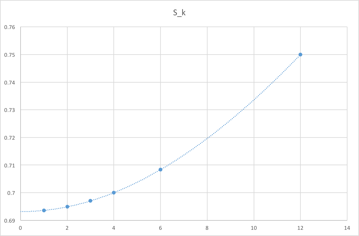
In his paper [Kramp 1815a], Kramp used \(N=12\), so that \(S(x)\) was a polynomial of degree 10
and the estimates \(S_1\), \(S_2\), \(S_3\), \(S_4\), \(S_6\) and \(S_{12}\) were fitted to the curve; see figure 7. This gave him an estimate
\[ \int_1^2 \frac{1}{x} dx \approx 0.69314806, \]
which has an absolute error of about \(8.8 \times 10^{-7}\), a little more than one part in a million of the true value. This is an impressively accurate estimate!
 |
Exercises for Students
- Use Kramp's algorithm to estimate \[ \int_0^1 \frac{1}{1+x^2} dx = \frac{\pi}{4} \] with \(N=4\). The steps are the same as in the first example above: calculate \(S_4\), \(S_2\), and \(S_1\), then fit the data to the curve \(S(x)=A + Bx^2 + Cx^4\), and use the value of \(A\) to approximate the integral.
You should find the approximate value to be \(\frac{6677}{8500}\). You don't need to use rational number arithmetic—floating point is just fine, but be sure to use plenty of digits of accuracy, say 8 at least. What is the absolute error in this estimate? - The integral in the exercise #1 is not the only way to estimate the value of \(\frac{\pi}{4}\). Repeat the steps of exercise #1 to estimate the definite integral \[ \int_0^1 \sqrt{1-x^2} \, dx. \] Of course, it's not possible to do this using rational number arithmetic, so floating point calculations are the only reasonable option. Which of these two estimates of \(\frac{\pi}{4}\) is more accurate?
(Although Kramp himself estimated the integral in exercise #1 in [Kramp 1815a], he did not consider expression in this exercise. Since he had to do all of his calculations by hand, the appearance of a square root would have made the problem an order of magnitude more difficult.) - Here is one more definite integral whose exact value involves \(\pi\). \[ \int_0^1 \frac{1}{\sqrt{1-x^2}} dx. = \arcsin(1) = \frac{\pi}{2} \] Can Kramp's algorithm be used to estimate this integral? What about the integral \[ \int_0^{\frac12} \frac{1}{\sqrt{1-x^2}} dx. = \arcsin(1) = \frac{\pi}{6}? \]
- Use Kramp's algorithm to give an estimate of \[ \int_1^2 \frac{1}{x} dx \] with \(N=6\). This will give you values of \(S_6\) when \(\Delta x = 1\), \(S_3\) when \(\Delta x = \frac{1}{2}\), \(S_2\) when \(\Delta x = \frac{1}{3}\), and \(S_1\) when \(\Delta x =\frac{1}{6}\). You will fit four data points to the equation \[ S(x) = A + Bx^2 + Cx^4 + Dx^6 \] and use the value of \(A\) to estimate the integral. You will probably want to use some sort of software package to solve the resulting \(4 \times 4\) linear system.
- Repeat exercise #1 with \(N=6\).
- Repeat exercise #2 with \(N=6\).
- Repeat exercise #4 with \(N=10\). Intuitively, this might be expected to give about the same level of accuracy as \(N=6\), because it also involves four estimates: \(S_{10}\), \(S_5\), \(S_2\) and \(S_1\). On the other hand, we expect \(S_1\) to be more accurate in this case because it uses \(n=10\) subintervals instead of only 6. Which estimate is more accurate?
- Repeat exercise #1 with \(N=10\).
- Repeat exercise #2 with \(N=10\).
- As a challenge problem, repeat exercises #4 and #1 with \(N=12\). These are the results given by Kramp in his paper [Kramp 1815a]. His results were 0.69314806 and 0.78539271, respectively.
Robert E. Bradley (Adelphi University) and Salvatore J. Petrilli, Jr. (Adelphi University), "Servois' 1817 "Memoir on Quadratures" – Student Exercises on The Trapezoidal Rule and Kramp's Algorithm," Convergence (May 2019)


