The Four Curves of Alexis Clairaut: Descartes’ Geometrie

As noted in the previous section, René Descartes (1596–1650) was one of several early modern mathematicians who revisited the ancient solutions to the problem of constructing mean proportionals. In his 1637 La Géométrie, Descartes criticized (in an indirect way) Greek mathematicians for the complicated nature of their solutions to this problem. At the beginning of Book III, he revisited his mesolabe compass, a pseudo-mechanical device which he described in Book II. This device, he believed, provides the easiest manner of finding any number of means:

For example, there is, I believe, no easier method of finding any number of mean proportionals, nor one whose demonstration is clearer, than the one which employs the curves described by the instrument \(XYZ\), previously explained. [3, p. 155]

Descartes’ mesolabe compass, which he called “instrument \(XYZ\)”, consists of a number of sliding straightedges linked together. One straightedge, \(YZ\), remains fixed and, in the diagram below, horizontal. Another straightedge, \(YX\), is attached to \(YZ\) with a hinge at \(Y\). A point \(A\) is chosen on the horizontal segment \(YZ\), with \(B\) chosen to be at the same distance from \(Y\) as \(A\) is. As the hinge is opened, the point \(B\) traces out an arc of a circle.

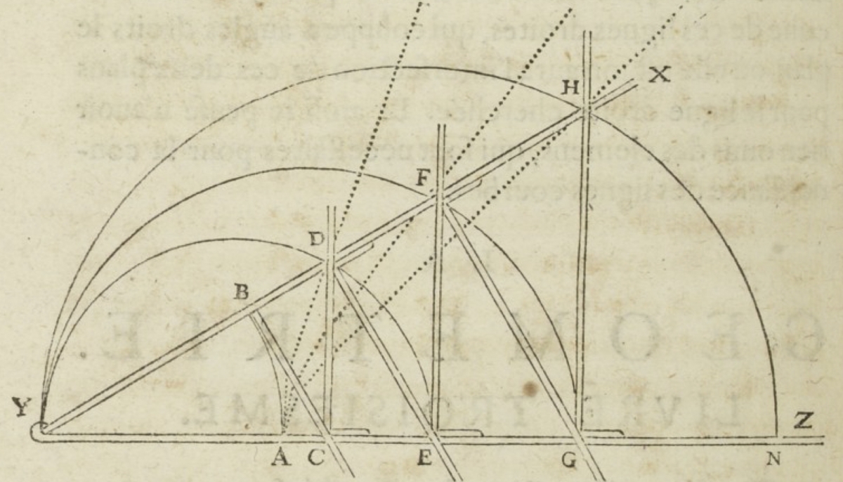
Figure 2: Descartes’ Mesolabe Compass, [3, pp. 46, 154]. gallica.bnf.fr / Bibliothèque nationale de France.

At \(B\), a perpendicular segment \(BC\) is drawn, and the point at which it intersects the horizontal \(YZ\) is marked as \(C\). A perpendicular to the horizontal is drawn from \(C\), intersecting the segment \(YX\) at \(D\). This process of dropping a perpendicular from \(YX\) and then drawing a perpendicular from \(YZ\) can be performed as many times as one wishes: Descartes’ diagram has three downward perpendiculars and three vertical perpendiculars.

As the hinge is opened, the point \(B\) induces a movement of the other intersection points. If we track the movement of \(D\), for example, a curve is traced out. Letting the radius \(YA = a\), we can find the equation for this curve:

\(x^4 = a^2(x^2 + y^2)\),

which is the same as Clairaut’s first curve (with one exception: Clairaut gave \(y^4 = a^2(x^2 + y^2)\), but this merely exchanges the \(x\) and \(y\) axes; see Editorial Conventions: General below for more on this issue). Descartes himself did not explicitly give the equations for the curves traced by \(D\), \(F\), or \(H\), but these are