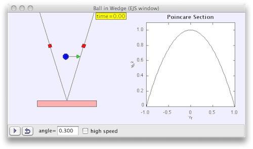
Figure 1. Example EJS program that simulates the path of a ball confined between two walls.
by Tim Chartier and Erich Kreutzer, Davidson College
An important component of software's success is an inviting and intuitive interface. Graphics and animation often engage a user. However, such features can be the most time-consuming and difficult portions to add to programs. In this article, we introduce and review Easy Java Simulations software, often abbreviated EJS. We will discuss its striking benefits and also its limitations. Most of all, we will see how EJS can do the heavy-lifting of adding graphical user interfaces (GUIs) to your computer programs.
EJS is a software tool created to help science teachers and students with little or no programming background easily visualize scientific phenomena. Although the freeware application caters to scientific simulations, EJS can be applied to a wide variety of concepts. Simulations that result from programming with EJS can be quite complex, often masking the ease of the process involved in their creation. As an initial example, let us view a simulation available at Open Source Physics. The image in Figure 1 is a screenshot of an EJS simulation modeling the path of a ball confined to move between two walls that form a wedge shape.
Effectively using EJS, at least in the beginning, will likely require some initial reading. To get started, you should reference the OSP EJS Modeling Overview, which includes an introduction to EJS and a discussion on the relationship between EJS and Java. This online resource can serve as an important primer. It leads the reader through a simple example while explaining the general philosophy behind EJS, which, in short, is that EJS splits the simulation into three parts. The first focuses on writing a description of what will happen in the simulation. The second part allows you to define variables and describe how they change over time. Finally, to complete the simulation, you define the visualization. Although this may seem complex, in actual use, EJS is very simple. For this reason we will walk you through the steps to create a program.
Let us examine the Lotka-Volterra predator prey model. This simple differential equation model starts with two variables, x denoting the population of prey, and y denoting the population of predators. There are then four more parameters: A denotes the growth rate of the prey when there is no predation, C denotes the decay rate of predators when there is no prey, B denotes the rate at which predators destroy prey, and finally D denotes the rate at which the predator population increases from consuming prey. These variables form the system of differential equations: dx/dt = Ax - Bxy and dy/dt = -Cy + Dxy.
Now we will create a simple visualization of the two populations versus time using EJS. After launching, we move to the Model portion of the interface. This is where we enter the variables for our simulation. Follow the directions and click to create a new page of variables. After giving the page a name, you add the variables described in the model. Variables are added by directly editing the variable table that was just created. Figure 2 shows this step for our example.

The next step in creating our simulation is to describe how the model changes over time. Since we are using a differential equation model you need to move to the Evolution portion and create a page of ODEs. After naming the page, indicate the independent variable, t, and then enter the differential equations for the model. The equations can be inserted by double-clicking the table cells. For our example, this leads to the resulting window seen in Figure 3.

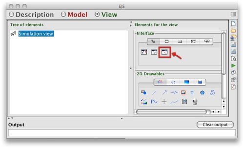
Having defined the model, we move to the visualization. Our goal is to see how the predator and prey populations vary with time. Thus, we want to create a plot of x and y versus t. So, we add a plot to our visualization window. You accomplish this by clicking the PlottingFrame element highlighted below and then clicking Simulation View in the Tree of Elements.
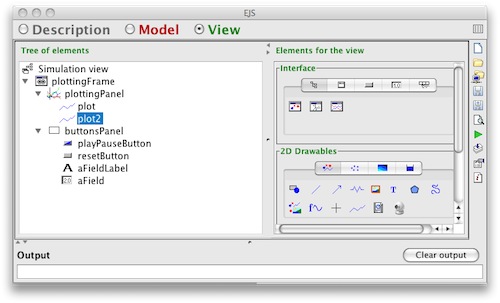
Next, we indicate what variables the plot will graph. By double clicking plot within the Tree of Elements, a new window pops up. Fill the Input X and Input Y fields with t and x respectively. To help differentiate the two populations, edit the Line Color parameter to be BLUE. Next we add a plot of the predator versus time by right-clicking the plot just edited and selecting Copy from the popup menu. Then right-click the plottingPanel element and select Paste. Edit the plot2 element so that Input Y is y. After completing these steps, your window should look like Figure 5.
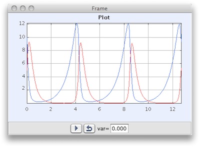
In those short steps, a complete simulations is ready for use. Indeed, it is easy to visualize such a model with EJS. To see your resulting work, click the green triangle on the right side of the main window to launch and see the application, which should resemble Figure 6.
The simulation may seem limited as the values for the variables are not editable. With a little more work you can add the ability to change the parameters. The updated applet appears in Figure 7 for your use. To alter the parameters simply reset the animation, change a value, and press enter. Then you can play the simulation and see what happens.
Having seen how simple it can be to create interactive simulations with EJS, let us view other examples to broaden our perspective of the programming possibilities with EJS. Again, models governed by differential equations can be especially easy to create in EJS. We've seen the Lotka-Volterra predator prey model in Figure 7. The application in Figure 1 simulates a ball's trajectory within a wedge formed by two walls. This again results from the entry of differential equations although the presence of the walls does require more Java programming. Figure 8 contains an applet of this simulation which again allows ample opportunities for exploration. To learn more about the simulation, right-click the graph and select Show Description.
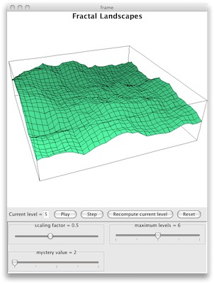
Simulations need not be continuous models defined by differential equations. Such examples may require more Java programming, but can be as complex and visually captivating as their continuous counterparts. In Figure 9, we see a screenshot of an applet that enables a user to create fractal landscapes. This example showcases three dimensional plotting. The example is extracted from a larger article, Mountains of Fractals, which packages multiple applications along with accompanying text and graphics into a single application that can be downloaded and launched on computers of various platforms. This demonstrates one of the powerful tools within EJS, the ability to package writing and multiple simulations into a single distribution piece.
Another great feature of EJS is the ability to look at the source code of any EJS applications (unfortunately, this feature does not work for applets within websites). This allows you to see what was necessary to create the behavior in the examples. To do this, you simply right-click on a plot and select the Open Ejs Model item. This will open the model in EJS after asking you to save the file to disk. Thus, whenever you find an application with a feature you would like to add to your simulation, you can see how it was accomplished.
Given the ease and power of programming with EJS, it is natural to want to distribute your resulting work. Completed programs can be placed in webpages as applets, as we have already seen in this article, or collected into a JAR file, a self-launching application that a user downloads and runs. These are quite different techniques for sharing your work and both are easily accomplished with EJS.
Instructing EJS to create a webpage that contains and runs one or more EJS simulations as applets requires only a few clicks. Generally, the web page serves as a skeleton for the final page as the text is minimal. Still, EJS compiles the simulation into a format that can be loaded from within a web page. You are left only needing to add necessary text and images to suit your needs. In fact, the applets you have viewed within this article were produced in this very way, with the text you are currently reading being added at a later time.
The other powerful export option presented by EJS uses another Java tool, the Open Source Physics Launcher (OSP Launcher). This tool, which comes packaged with EJS, allows you to combine text and simulations into one hierarchical application. The benefit of having one package is that the user only has to download one file to get the entire activity. One downside is that the OSP Launcher can be complex. The online documentation can help a user learn to effectively utilize OSP Launcher's options. As an example you can use the link provided in Figure 9 to download the JAR file containing the Mountains of Fractals article. Again, notice the integration of text and applications within one downloadable file.
EJS can be an extremely useful tool when producing simulations, but, as with any software, there are limitations to keep in mind. Documentation can be lacking at times. For the commonly used interface objects, documentation includes simple informative example projects. For more complex and less frequently used interface objects, however, the documentation is more sparse. Fortunately there is a library of examples that uses a variety of the features and perusing this body of examples can often enable you to find an example that utilizes a desired feature.
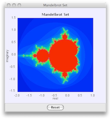
The inherent generational paradigm can also prove challenging, depending on your programming goals. EJS assumes that the simulation will be time or generational dependent. For most applications this works well, but as in the Mandelbrot example in Figure 10 below, the code becomes more complex when that paradigm does not fit. Again, simulations based on differential equations may require only a few steps with EJS to produce the resulting program and may not require much expertise in Java programming. For programs that are not based on differential equations, Java code may need to be added, which EJS allows, and one should reference the documentation for more information.
Producing simulations can be surprisingly simple with EJS. Yet, if you have very specific user interface needs or desire a specific "look" for your application, then you may be required to do more programming. Such cases generally require tweaking display properties of numerous interface components. Given the sparse documentation for some display properties, trial and error often ensues. While this may not be a limitation for some, it may be for others and should be kept in mind if someone comes to EJS with very specific programming needs in mind.
EJS is a powerful tool that you may want to consider adopting for creating Java applications. You may be able to introduce it to your students who may or may not have much programming experience. As we have seen with the limited number of applets in this article, EJS can produce attractive simulations that allow user interaction. There are some limitations, but one should also keep in mind that EJS continues to be developed and new versions often offer useful new features. These new versions also hint at improved support and documentation in the near future. From our experience, EJS can produce quality simulations much more quickly than starting from scratch. Now, it's time for you to jump into programming with EJS, if it interests you, and visit the download page to get the current version. It is just that easy to get started with EJS.