Visualizing Lie Subalgebras using Root and Weight Diagrams
Aaron Wangberg
Department of Mathematics
Winona State University University
Winona, MN 55987
awangberg@winona.edu
Tevian Dray
Department of Mathematics
Oregon State University
Corvallis, OR 97331
tevian@math.oregonstate.edu
Abstract
While Dynkin diagrams are useful for classifying Lie algebras, it is the root and weight diagrams that are most often used in applications, such as when describing the properties of fundamental particles. This paper illustrates how to construct root and weight diagrams from Dynkin diagrams, and how the root and weight diagrams can be used to identify subalgebras. In particular, we show how this can be done for some algebras whose root and weight diagrams have dimension greater than 3, including the exceptional Lie algebras \(F_4\) and \(E_6\).
Contents
- Abstract
- Contents
- 1. Introduction
- 2. Root and Weight Diagrams of Lie Algebras
- 3. Subalgebras of Algebras
- 4. Applications to Algebras of Dimension Greater than 3
- 5. Conclusion
- Endnotes
- References
This article uses jsMath, which requires JavaScript, to process the mathematics expressions. If your browser supports JavaScript, be sure it is enabled. Once the jsMath scripts are running, clicking the "jsMath" button in the lower right corner of the browser window brings up a panel with configuration options and links to documentation and download pages, including instructions for installing missing mathematics fonts. This article also uses JavaView for 3-D graphics and animations, so be sure you have a recent Java plug-in installed for your browser. In figures with 3-D graphics (indicated by axis vectors in the lower left corner of the figure), the object shown can be rotated by clicking and dragging the mouse on the graph. In some figures, a "Keyframe Animation" panel will appear in a new window, providing controls for animated figures.
For readers who prefer to view the article offline, it is available for download in a compressed ZIP archive (13.9 Mb compressed, 24.3 Mb uncompressed). After downloading the archive, unpack it using a compression utility such as 7-Zip, then in the uncompressed folder open the file "joma_article.pdf" using a PDF reader such as Adobe Acrobat Reader. The graphics in the article file are all static, but include links to HTML files in the folder which provide the interactive versions of the graphics.
Published February 2009. © 2009 Aaron Wangberg and Tevian Dray.
Visualizing Lie Subalgebras using Root and Weight Diagrams
1. Introduction
Lie algebras are classified using Dynkin diagrams, which encode the geometric structure of root and weight diagrams associated with an algebra. This paper begins with an introduction to Lie algebras, roots, and Dynkin diagrams. We then show how Dynkin diagrams define an algebra's root and weight diagrams, and provide examples showing this construction. In Section 3, we develop two methods to analyze subdiagrams. We then apply these methods to the exceptional Lie algebra \(F_4\), and describe the slight modifications needed in order to apply them to \(E_6\). We conclude by listing all Lie subalgebras of \(E_6\).
2. Root and Weight Diagrams of Lie Algebras
We summarize here some basic properties of root and weight diagrams. Further information can be found in [1], [2], and [3]. A description of how root and weight diagrams are applied to particle physics is also given in [2].
2.1 Lie Algebras
A Lie algebra \(g\) of dimension \(n\) is an \(n\)-dimensional vector space along with a product \([\ ,\ ]:g \times g \to g\), called a commutator, which is anti-commutative (\([x,y] = -[y,x]\)) and satisfies the Jacobi Identity $$[x,[y,z]] + [y,[z,x]] + [z,[x,y]] = 0$$ for all \(x,y,z \in g\). A Lie algebra is called simple if it is non-abelian and contains no non-trivial ideals. All complex semi-simple Lie algebras are the direct sum of simple Lie algebras. Thus, we follow the standard practice of studying the simple algebras, which are the building blocks of the semi-simple algebras.
There are four infinite families of Lie algebras as well as five exceptional Lie algebras. The (compact, real forms of) the algebras in the four infinite families correspond to special unitary matrices (or their generalizations) over different division algebras. The algebras \(B_n\) and \(D_n\) correspond in this way to real special orthogonal groups in odd and even dimensions, \(SO(2n+1)\) and \(SO(2n)\), respectively. The algebras \(A_n\) correspond to complex special unitary groups \(SU(n+1)\), and the algebras \(C_n\) correspond to unitary groups \(SU(n,\mathbb{H})\) over the quaternions, which are more usually described as (some of the) symplectic groups.
While Lie algebras are usually classified using their complex representations, there are particular real representations, based upon the division algebras, which are of interest in particle physics. Manogue and Schray [4] describe the use of quaternions \(\mathbb{H}\) to construct \(su(2,\mathbb{H})\) and \(sl(2, \mathbb{H})\), which are real representations of \(B_2=so(5)\) and \(D_3 = so(5,1)\), respectively. As they discuss, their construction naturally generalizes to the octonions \(\mathbb{O}\), yielding the real representations \(su(2,\mathbb{O})\) and \(sl(2,\mathbb{O})\) of \(B_4 = so(9)\) and \(D_5 = so(9,1)\), respectively. This can be further generalized to the \(3 \times 3\) case, resulting in \(su(3,\mathbb{O})\) and \(sl(3, \mathbb{O})\), which preserve the trace and determinant, respectively, of a \(3 \times 3\) octonionic hermitian matrix, and which are real representations of two of the exceptional Lie algebras, namely \(F_4\) and \(E_6\), respectively [5]. The remaining three exceptional Lie algebras are also related to the octonions [6, 7]. The smallest, \(G_2\), preserves the octonionic multiplication table and is 14-dimensional, while \(E_7\) and \(E_8\) have dimensions 133 and 248, respectively. A major stem in describing the infinite-dimensional unitary representation of the split form of \(E_8\) was recently completed by the Atlas Project [8].
In sections 2 and 3, we label the Lie algebras using their standard name (e.g. \(A_n\), \(B_n\)) and also with a standard complex representation (e.g. \(su(3)\), (so(7))). In section 4, when discussing the subalgebras of \(E_6\), we also give particular choices of real representations.
2.2 Roots and Root Diagrams
Every simple Lie algebra \(g\) contains a Cartan subalgebra \(h \subset g\), whose dimension is called the rank of \(g\). The Cartan subalgebra \(h\) is a maximal abelian subalgebra such that \(ad H\) is diagonalizable for all \(H \in h\). The Killing form can be used to choose an orthonormal basis \(\{h_{1}, \cdots, h_{l}\}\) of \(h\) which can be extended to a basis \[\{ h_{1}, \cdots, h_{l}, g_1, g_{-1}, g_2, g_{-2},\cdots, g_{\frac{n-l}{2}}, g_{-\frac{n-l}{2}} \} \] of \(g\) satisfying:
- \([h_{i}, g_{j}] = \lambda_i^j g_{j}\) (no sum), \(\lambda_i^j \in \mathbb{R}\)
- \([h_{i}, h_{j}] = 0 \)
- \([g_{j}, g_{-j}] \in h\)
The basis elements \(g_j\) and \(g_{-j}\) are referred to as raising and lowering operators. Property 1 associates every \(g_{j}\) with an \(l\)-tuple of real numbers \(r^{j} = \langle\lambda_1^j, \cdots, \lambda_l^j\rangle\), called roots of the algebra, and this association is one-to-one. Further, if \(r^{j}\) is a root, then so is \(-r^{j} = r^{-j}\), and these are the only two real multiples of \(r^{j}\) which are roots. According to Property 2, each \(h_i\) is associated with the \(l\)-tuple \(\langle0, \cdots, 0\rangle\). Because this association holds for every \(h_i \in h\), these \(l\)-tuples are sometimes referred to as zero roots. For raising and lowering operators \(g_j\) and \(g_{-j}\), Property 3 states that \(r^{j} + r^{-j} = \langle0, \cdots, 0\rangle\).
Let \(\Delta\) denote the collection of non-zero roots. For roots \(r^{i}\) and \(r^{j} \ne -r^i\), if there exists \(r^{k} \in \Delta\) such that \(r^i + r^j = r^k\), then the associated operators for \(r^i\) and \(r^j\) do not commute, that is, \([ g_i, g_j ] \ne 0\). In this case, \([g_i, g_j] = C^{k}_{ij}g_{k}\) (no sum), with \(C^k_{ij} \in \mathbb{C}, C^i_{ij} \ne 0\). If \(r^i + r^j \not\in \Delta\), then \([g_i, g_j] = 0\).
When plotted in \(\mathbb{R}^l\), the set of roots provide a geometric description of the algebra. Each root is associated with a vector in \(\mathbb{R}^l\). We draw \(l\) zero vectors at the origin for the \(l\) zero roots corresponding to the basis \(h_1, \cdots, h_l\) of the Cartan subalgebra. For the time being, we then plot each non-zero root \(r^i = \langle\lambda_1^i, \cdots, \lambda_l^i\rangle\) as a vector extending from the origin to the point \(\langle\lambda_1^i, \cdots, \lambda_l^i\rangle\). The terminal point of each root vector is called a state. As is commonly done, we use \(r^i\) to refer to both the root vector and the state. In addition, we allow translations of the root vectors to start at any state, and connect two states \(r^i\) and \(r^j\) by the root vector \(r^k\) when \(r^k + r^i = r^j\) in the root system. The resulting diagram is called a root diagram.
As an example, consider the algebra \(su(2)\), which is classified as \(A_1\). The algebra \(su(2)\) is the set of \(2 \times 2\) complex traceless Hermitian matrices. Setting
| \[ \sigma_1 = \left[ \begin{array}{cc} 0 & 1 \\ 1 & 0 \\ \end{array} \right] \] | \[ \sigma_2 = \left[ \begin{array}{cc} 0 & -i \\ i & 0 \\ \end{array} \right] \] | \[ \sigma_3 = \left[ \begin{array}{cc} 1 & 0 \\ 0 & -1 \\ \end{array} \right] \] |
we choose the basis \(h_1 = \frac{1}{2}\sigma_3\) for the Cartan subalgebra \(h\), and use \(g_1 = \frac{1}{2}(\sigma_1+i\sigma_2)\) and \(g_{-1} = \frac{1}{2}(\sigma_1-i\sigma_2)\) to extend this basis for all of \(su(2)\). Then
- \([h_1, h_1] = 0\)
- \([h_1, g_1] = 1 g_1\)
- \([h_1, g_{-1}] = -1 g_{-1}\)
- \([g_{1}, g_{-1}] = h_1\)
By Properties 2 and 3, we associate the root vector \(r^1 = \langle1\rangle\) with the raising operator \(g_1\) and the root vector \(r^{-1} = \langle-1\rangle\) with the lowering operator \(g_{-1}\). Using the zero root \(\langle0\rangle\) associated with \(h_1\), we plot the corresponding three points \((1)\), \((-1)\), and \((0)\) for the states \(r^1\), \(r^{-1}\), and \(h_1\). We then connect the states using the root vectors. Instead of displaying both root vectors \(r^1\) and \(r^{-1}\) extending from the origin, we have chosen to use only the root vector \(r^{-1}\), as \(r^{-1} = - r^{1}\), to connect the states \((1)\) and \((0)\) to the states \((0)\) and \((-1)\), respectively. The resulting root diagram is illustrated in Figure 1.
 |
|
|
Visualizing Lie Subalgebras using Root and Weight Diagrams
2.3 Weights and Weight Diagrams
An algebra \(g\) can also be represented using a collection of \(d \times d\) matrices, with \(d\) unrelated to the dimension of \(g\). The matrices corresponding to the basis \(h_1, \cdots, h_l\) of the Cartan subalgebra can be simultaneously diagonalized, providing \(d\) eigenvectors. Then, a list \(w^m\) of \(l\) eigenvalues, called a weight, is associated with each eigenvector. Thus, the diagonalization process provides \(d\) weights for the algebra \(g\). The roots of an \(n\)-dimensional algebra can be viewed as the non-zero weights of its \(n \times n\) representation.
Weight diagrams are created in a manner comparable to root diagrams. First, each weight \(w^i\) is plotted as a point in \(\mathbb{R}^l\). Recalling the correspondence between a root \(r^i\) and the operator \(g^i\), we draw the root \(r^k\) from the weight \(w^i\) to the weight \(w^j\) precisely when \(r^k + w^i = w^j\), which at the algebra level occurs when the operator \(g^k\) raises (or lowers) the state \(w^i\) to the state \(w^j\).
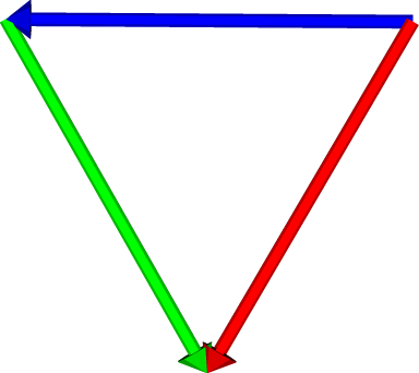
The root and minimal non-trivial weight diagrams of the algebra \(A_2 = su(3)\) are shown in Figure 2.1 The algebra has three pairs of root vectors, which are oriented east-west (colored blue), roughly northwest-southeast (colored red), and roughly northwest-southeast (colored green). The algebra's rank is the dimension of the underlying Euclidean space, which in this case is \(l=2\), and the number of non-zero root vectors is the number of raising and lowering operators. The minimal weight diagram contains six different roots, although we've only indicated one of each raising and lowering root pair. Using the root diagram, the dimension of the algebra can now be determined either from the number of non-zero roots or from the number of root vectors extending in different directions from the origin. Both diagrams indicate that the dimension of \(A_2 = su(3)\) is \(8 = 6+2\). A complex semi-simple Lie algebra can almost2 be identified by its dimension and rank. We note that the algebra's root system, and hence its root diagram or weight diagram, does determine the algebra up to isomorphism.
 |
 |
|
|
|
||
2.4 Constructing Root Diagrams from Dynkin Diagrams
In 1947, Eugene Dynkin simplified the process of classifying complex semi-simple Lie algebras by using what became known as Dynkin diagrams [9]. As pointed out above, the Killing form can be used to choose an orthonormal basis for the Cartan subalgebra. Then every root in a rank \(l\) algebra can be expressed as an integer sum or difference of \(l\) simple roots. Further, the relative lengths and interior angle between pairs of simple roots fits one of four cases. A Dynkin diagram records the configuration of an algebra's simple roots.
Each node in a Dynkin diagram represents one of the algebra's simple roots. Two nodes are connected by zero, one, two, or three lines when the interior angle between the roots is \(\frac{\pi}{2}\), \(\frac{2\pi}{3}\), \(\frac{3\pi}{4}\), or \(\frac{5\pi}{6}\), respectively. If two nodes are connected by \(n\) lines, then the magnitudes of the corresponding roots satisfy the ratio \(1:\sqrt{n}\). An arrow is used in the Dynkin diagram to point toward the node for the smaller root. If two roots are orthogonal, no direct information is known about their relative lengths.
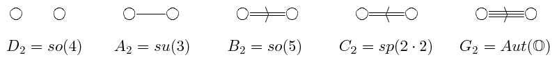
We give the Dynkin diagrams for the rank 2 algebras in Figure 3 and the corresponding simple root configurations in Figure 4. For each algebra, the left node in the Dynkin diagram corresponds to the root \(r^1\) of length 1, colored red and lying along the horizontal axis, and the right node corresponds to the other root \(r^2\), colored blue.
 |
|
|
 |
||||
|
|
|
|
|
|
|
|
||||
In \(\mathbb{R}^l\), each root \(r^i\) defines an \((l-1)\)-dimensional hyperplane which contains the origin and is orthogonal to \(r^i\). A Weyl reflection for \(r^i\) reflects each of the other roots \(r^j\) across this hyperplane, producing the root \(r^k\) defined by $$r^k = r^j - 2(\frac{r^j {\tiny \bullet} r^i}{|r^i|})\frac{r^i}{|r^i|} $$ According to Jacobson [1], the full set of roots can be generated from the set of simple roots and their associated Weyl reflections.
We illustrate how the full set of roots can be obtained from the simple roots using Weyl reflections in Figure 5. We start with the two simple roots for each algebra, as given in Figure 4. For each algebra, we refer to the horizontal simple root, colored red, as \(r^1\), and the other simple root, colored blue, as \(r^2\). Step 1 shows the result of reflecting the simple roots using the Weyl reflection associated with \(r^1\). In this diagram, the black thin line represents the hyperplane orthogonal to \(r^1\), and the new resulting roots are colored green. Step 2 shows the result of reflecting this new set of roots using the Weyl reflection associated with \(r^2\). At this stage, both \(D_2 = so(4)\) and \(A_2 = su(3)\) have their full set of roots. We repeat this process again in steps 3 and 4, using the Weyl reflections associated first with \(r^1\) and then with \(r^2\). The full root systems for \(B_2 = so(5)\) and \(C_2 = sp(2\cdot 2)\) are obtained after the three Weyl reflections. Only \(G_2\) requires all four Weyl reflections.
|
|
|
|
 |
|
 |
 |
 |
||||
|
|
|
|
|
|
||||
|
|
||||||||
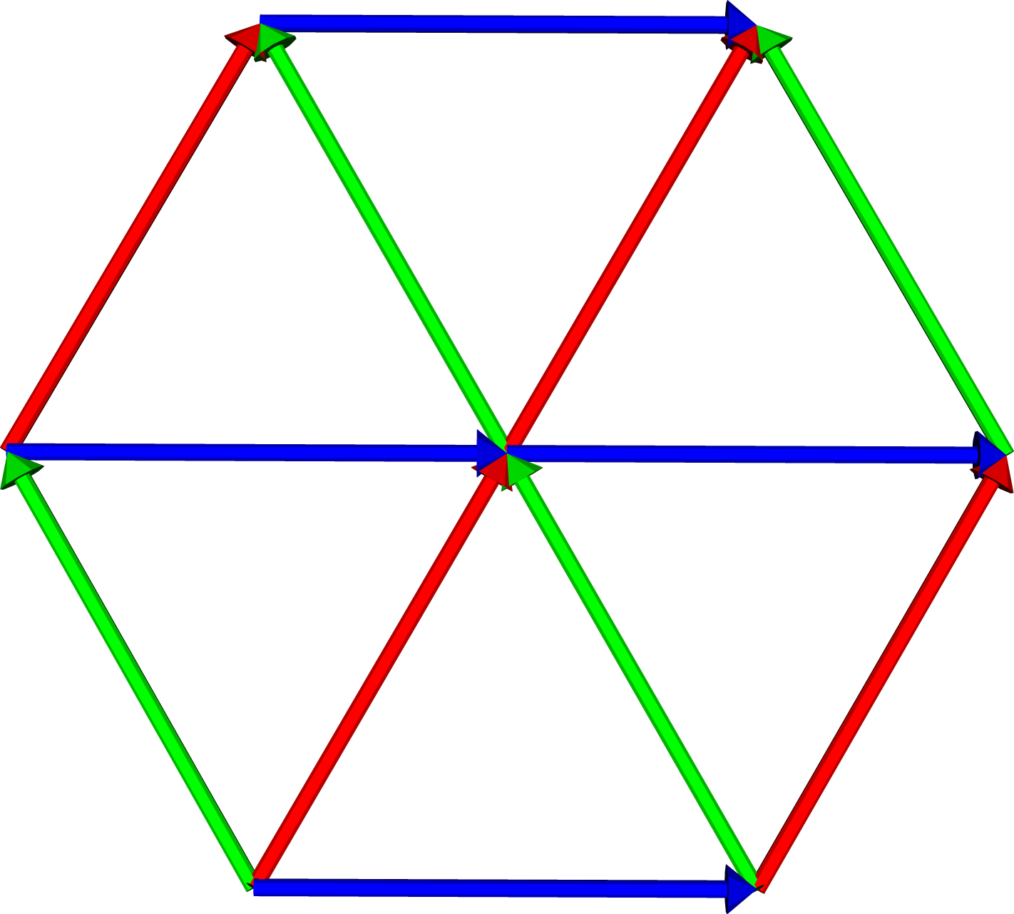
The full set of roots have been produced once the Weyl reflections fail to produce additional roots. The root diagrams are completed by connecting vertices \(r^i\) and \(r^j\) via the root \(r^k\) precisely when \(r^k + r^i = r^j\). From the root diagrams in Figure 6, it is clear that the dimension of \(A_2=su(3)\) is 8 and the dimension of \(G_2\) is 14, while both \(B_2=so(5)\) and \(C_2=sp(2\cdot 2)\) have dimension \(10\). Further, since the diagram of \(B_2\) can be obtained via a rotation and rescaling of the root diagram for \(C_2\), it is clear that \(B_2\) and \(C_2\) are isomorphic.
Visualizing Lie Subalgebras using Root and Weight Diagrams
2.5 Constructing Weight Diagrams from Dynkin Diagrams
Root diagrams are a specific type of weight diagram. While the states and roots can be identified with each other in a root diagram, this does not happen for general weight diagrams. Weight diagrams are a collection of states, called weights, and the roots are used to move from one weight to another. Although it has only one root diagram, an algebra has an infinite number of weight diagrams.
Like a root diagram, any one of an algebra's weight diagrams can be constructed entirely from its Dynkin diagram. The Dynkin diagram records the relationship between the \(l\) simple roots of a rank \(l\) algebra. Each simple root \(r^1, \cdots, r^l\) is associated with a weight \(w^1, \cdots, w^l\). When all integer linear combinations of these weights are plotted in \(\mathbb{R}^l\), they form an infinite lattice of possible weights. This lattice contains every weight from every \(d \times d\) \((d \ge 0)\) representation of the algebra. These weights may be ordered. Every weight diagram then contains a highest weight \(W\) which satisfies \(W > W_i\) for every other weight \(W_i\) in the diagram. Alternatively, a diagram's highest weight \(W\) is an element of the boundary \(\overline{W}\) of the set of all weights in the diagram; \(\overline{W}\) contains all the weights in the diagram which are furthest from the origin. A particular weight diagram is chosen by selecting a weight \(W\). Weyl reflections related to the weights \(w^1, \cdots, w^l\) determine the weights in \(\overline{W}\) for the weight diagram. To determine the diagram's weights in the interior of \(\overline{W}\), we note that valid weights must be connected by the algebra's roots. Hence, all of the weights within \(\overline{W}\) which are integer linear combinations of the roots away from the weights in \(\overline{W}\) are valid and should be a part of the diagram. Having selected all of the diagram's valid weights, we complete the diagram by connecting pairs of weights with root vectors.3 Choosing a new weight \(W\) outside the original weight diagram's boundary \(\overline{W}\) selects a new, larger, weight diagram. A smaller weight diagram is created by selecting a weight contained in the interior of \(\overline{W}\).
An equivalent method [10] constructs weight diagrams while avoiding the explicit use of Weyl reflections. First, the \(l\) simple roots \(r^1, \cdots, r^l\) are used to define the Cartan matrix \(A\), whose components are \(a_{ij} = 2 \frac{r^i {\tiny \bullet} r^j}{r^i {\tiny \bullet} r^i}\). Equivalently, the components are: \[ a_{ij} =\begin{cases} 2, &\text{if $i = j$;}\\ 0, &\text{if $r^i$ and $r^j$ are orthogonal;}\\ -3, &\text{if the interior angle between $r^i$ and $r^j$ is $\frac{5\pi}{6}$, and $\sqrt{3}|r^i| = |r^j|$;}\\ -2, &\text{if the interior angle between roots $r^i$ and $r^j$ is $\frac{3\pi}{4}$, and $\sqrt{2}|r^i| = |r^j|$;}\\ -1, &\text{in all other cases;}\\ \end{cases} \]
Cartan matrices are invertible. Thus, the fundamental weights \(w^1, \cdots, w^l\) defined by \[w^i = \sum_{k=1}^{l}(A^{-1})_{ki}r^k\] are linearly independent. We create an infinite lattice \(\mathbb{W} = \{ m_i w^i | m_i \in \mathbb{Z}\}\) of possible weights in \(\mathbb{R}^l\), and then label each weight \(W^i = m^i_j w^j \in \mathbb{W}\) using the \(l\)-tuple \(M^i = \left[m^i_1, \cdots, m^i_l\right]\), called a mark. We choose one of the infinite number of weight diagrams by specifying \(l\) non-negative integers \(m^0_1, \cdots, m^0_l\) for the mark of the highest weight \(W^0\).
While the components of the Cartan matrix record the geometry of the simple roots, the components of each mark record the geometric configuration of the weights within the lattice. Each weight (W^i) is part of a shell of weights \(\overline{W}\) which are equidistant from the origin. As discussed earlier, Weyl reflections associated with the fundamental weights can be used to find the weights in \(\overline{W}\). The diagram's entire set of valid weights can also be determined using the mark \(M^i\) of each weight. The positive integers \(m^i_j \in M^i\) list the maximum number of times that the simple root \(r^j\) can be subtracted from \(W^i\) while keeping the new weights on or within the boundary \(\overline{W}\). Thus, weights \(W^i - 1 r^j, \cdots, W^i - (m^i_j) r^j \textrm{ (no sum)}\) are valid weights occurring on or inside \(\overline{W}\). These new weights have marks \(M^i - A_i^{\it{T}}, M^i - 2 A_i^{\it{T}}, \cdots, M^i - m^i_j A_i^{\it{T}}\), where \(A_i^{\it{T}}\) is the transpose of the \(i\)-th column of the Cartan matrix \(A\). Thus, given a weight diagram's highest weight \(W^0\), this procedure selects all of the diagram's weights from the infinite lattice. The diagram is completed by connecting any two weights \(W^i\) and \(W^k\) by the root \(r^j\) whenever \(W^i + r^j = W^k\).
This procedure is carried out for the the algebra \(B_3=so(7)\), whose simple roots are \[ \begin{array}{ccc} r^1 = \langle\sqrt{2},0,0\rangle, & r^2 = \langle-\sqrt{\frac{1}{2}}, -\sqrt{\frac{3}{2}}, 0\rangle, & r^3 = \langle0, \sqrt{\frac{2}{3}}, \sqrt{\frac{1}{3}}\rangle \end{array} \] We produce the Cartan matrix \(A\), find \(A^{-1}\), and list the fundamental weights.
|
|
|
|
||
| $$ A = \left( \begin{array}{ccc} 2 & -1 & 0 \\ -1 & 2 & -1 \\ 0 & -2 & 2 \end{array} \right) $$ |
|
|
Starting with the highest weight \(W^0 = w^1\), whose mark is \(\left[1,0,0\right]\), the above procedure generates the following weights:
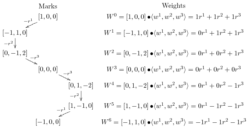
We plot the weight \(W^0, \cdots, W^6\) and the appropriate lowering roots \(-r^1, \cdots, -r^3\) at each weight for this weight diagram of \(B_3 = so(7)\) in Figure 7. The full set of roots are used to connect pairs of weights, giving the complete weight diagram of \(B_3 = so(7)\) in Figure 8.
|
|
|
|
|
|
|
2.6 Rank 3 Root and Weight Diagrams
Using the procedures outlined above, we catalog the root and minimal weight diagrams for the rank 3 algebras. We did this by writing a Perl program to generate the weight and root diagram structures and return executable Maple code. We then used Maple and Javaview to display the pictures.
The 3-dimensional root diagrams of the rank 3 algebras are given in Figure 9. The root diagrams of \(A_3=su(4)\) and \(D_3=so(6)\) are identical. Hence, \(A_3 = D_3\). These algebras have dimension 15, as their root diagram contains 12 non-zero states. The \(B_3=so(7)\) and \(C_3=sp(2\cdot 3)\) algebras both have dimension 21, and their root diagrams each contain 18 non-zero states. Each of these algebras contain the \(A_2=su(3)\) root diagram, which is a hexagon. This can be seen at the center of each rank 3 algebra by turning its root diagram in various orientations. The modeling kit ZOME [11] can be used to construct the rank 3 root diagrams. The kit contains connectors of the right length and nodes with the correct configuration of connection angles to construct all of the rank 3 root diagrams.
|
|
|
|
||
|
|
|
|
||
|
|
||||
An algebra's minimal weight diagram has the fewest number of weights while still containing all of the roots. Figure 10 shows the minimal weight diagrams for \(A_3=D_3\), \(B_3\), and \(C_3\). Each root occurs once in the diagram for \(A_3=D_3\), while in the diagram for \(B_3\) every root is used twice. The minimal weight diagram for \(C_3\) is centered about the origin, and the roots passing through the origin (colored red, blue, and brown) occur once, while the other roots occur twice.
|
|
|
|
||
|
|
|
|
||
|
|
||||
Visualizing Lie Subalgebras using Root and Weight Diagrams
3. Subalgebras of Algebras
We have already noted that we can recognize \(A_2 = su(3)\) as a subalgebra of \(A_3 = su(4)\), \(B_3 = so(7)\), and \(C_3 = sp(2\cdot 3)\) by identifying its hexagonal root diagram in each of the larger root diagrams. This section develops two further methods which help us identify subalgebras using root and weight diagrams. We emphasize that these methods are valid only when applied to the full root diagram, but not when applied to the root system alone.
3.1 Subalgebras of \(B_3=so(7)\) using Root Diagrams
Root and weight diagrams can be used to identify subalgebras. For algebras of rank \(l \le 3\), we can recognize subdiagrams corresponding to subalgebras by building the algebra's root and weight diagrams and rotating them in \(\mathbb{R}^3\).
We illustrate the process of finding all subalgebras of \(B_3=so(7)\) by using its root diagram. When rotated to the position in Figure 11, the large horizontal 2-dimensional rectangle through the origin (containing roots colored green and magenta) contains eight non-zero nodes. This subdiagram is the root diagram of the 10-dimensional algebra \(B_2 = C_2\). The smaller rectangular diagrams lying in parallel planes above and below this large rectangle contain all of the roots vectors of \(B_2=C_2\). These diagrams are minimal weight diagrams of \(B_2 = C_2\).
Two additional rotations of the root diagram of \(B_3=so(7)\) produce subalgebras. In Figure 12, the horizontal plane through the origin contains only two orthogonal roots, which are colored blue and fuchsia. These roots comprise the root diagram of \(D_2=su(2)+su(2)\). We have already identified the hexagonal \(A_2=su(3)\) root diagram in the horizontal plane containing the origin in Figure 13. Each horizontal triangle above and below this plane is a minimal weight representation of \(A_2\). In addition, the subdiagram containing the bottom triangle, middle hexagon, and top triangle is the 15-dimensional, rank 3 algebra \(A_3 = D_3\). Thus, it is possible to identify both rank \(l-1\) and rank \(l\) subalgebras of a rank \(l\) algebra.
|
|
|
|
||
|
|
|
|
||
|
|
||||
Not all subalgebras of a rank \(l\) algebra can be identified as subdiagrams of its root or weight diagram. When extending a rank \(l\) algebra to a rank \(l+1\) algebra, each root \(r^i = \langle \lambda_1^i, \cdots, \lambda_l^i \rangle\) is extended in \(\mathbb{R}^{l+1}\) to the roots \(r^{i_1}, \cdots, r^{i_m}\), where \(r^{i_j} = \langle \lambda_1^i, \cdots, \lambda_l^i, \lambda_{l+1}^{i_j} \rangle\). Here, \(\lambda_{l+1}^{i_j}\) is one of \(m \ge 1\) different eigenvalues values defined by the extension of the algebra. Hence, although roots \(r^{i_1}, \cdots, r^{i_m}\) are all distinct in \(\mathbb{R}^{l+1}\), they are the same root when restricted to their first \(l\) coordinates. Thus, we can identify subalgebras of a rank \(l+1\) algebra by projecting its root and weight diagrams along any direction.
Just as our eyes ``see'' objects in \(\mathbb{R}^3\) by projecting them into \(\mathbb{R}^2\), we can identify subalgebras of \(B_3=so(7)\) by projecting its root and weight diagram into \(\mathbb{R}^2\). In Figure 14 and Figure 15, we have rotated the root diagram of \(B_3\) so that our eyes project one of the root vectors onto another root vector. This method allows us to identify \(B_2=so(5)\) and \(G_2\) as subalgebras of \(B_3\) by recognizing their root diagrams in Figure 14 and Figure 15, respectively. Although we previously identified \(B_2 \subset B_3\) by using a subdiagram confined to a plane, we could not identify \(G_2\) as a subalgebra of \(B_3\) using that method.
|
|
|
|||
|
|
|
|||
|
|
||||
Visualizing Lie Subalgebras using Root and Weight Diagrams
3.2 Geometry of Slices and Projections
The procedures in subsections 2.4 and 2.5 allow us to create root and weight diagrams for algebras of rank greater than 3. We now give precise definitions for the two processes we used in subsection 3.1 to identify subalgebras of \(B_3 = so(7)\).
We first generalize the method that allowed us to find subalgebras of \(B_3=so(7)\) by identifying subdiagrams in specific cross-sections of its root diagram. We refer to this method as ``slicing'', based on an analogy to slicing a loaf of bread. A knife, making parallel cuts through the bread, creates several independent slices of the bread. We use the same idea to slice an algebra's root or weight diagram. A set of \(l-1\) linearly independent vectors \(V = \{v^1, \cdots, v^{l-1}\}\) defines an \((l-1)\)-dimensional hyperplane in \(\mathbb{R}^l\). Given \(V\), a slice \(D_{\alpha}\) of an algebra's \(l\)-dimensional diagram \(D\) is the subdiagram consisting of the vertex \(\alpha\) and all root vectors and vertices in the hyperplane spanned by \(V\) containing \(\alpha\). A slicing of a diagram \(D\) using \(V\) separates \(D\) into a finite set of disjoint slices. The root vectors which connect vertices from two different slices are called struts. We are interested in slices of \(D\) which contain diagrams corresponding to the algebra's subalgebras. Hence, the slices must contain root vectors of \(D\), and in practice we choose \(V\) to consist of integer linear combinations of simple roots.
A diagram's slices can tell us about its original structure. When dealing with bread, we can obviously stack the slices on top of each other, in order, to recreate an image of the pre-cut loaf of bread - our mind removes the cuts made by the knife. When dealing with root and weight diagrams, we do not have the benefit of using the shape of an ``outer crust'' to guide the stacking of the slices of the diagram. Instead of severing the struts, we color them grey to make them less prominent. This allows us to use the slices and struts to recreate the structure of the original root or weight diagram.
When the dimension of the diagram is greater than 3, stacking slices on top of each other is not an effective means of recreating the root or weight diagram. Instead, we lay the slices out along one direction, much as slices of bread are laid in order along a countertop to make sandwiches. This allows us to display a 3-dimensional diagram in two dimensions, as we have shown for \(B_3=so(7)\) in Figure 16, or a 4-dimensional diagram in three dimensions, as we have shown for the root diagram of \(B_4 =so(9)\) in Figure 17. Of course, a 5-dimensional diagram can be displayed in three dimensions by first laying 4-dimensional slices along the \(x\) axis, and then slicing each of these diagrams and spreading them along directions parallel to the \(y\) axis. This procedure generalizes easily to diagrams for rank six algebras, and can be modified to allow any compact \(n\)-dimensional diagram to be displayed in three dimensions.
 |
|
|
|
|
|
|
For the Lie algebras of rank \(l = 6\) or less, we implement a slicing as follows. We first build the algebra's root or weight diagram as described in subsection 2.5. Given three vectors \(v^1\), \(v^2\), and \(v^3\) to define the slicing, we apply an orthonormal transformation so that the slices are contained within the first 3 coordinates of \(\mathbb{R}^l\). We then use the projection (given here for \(l=6\)) \(\mathbb{R}^6 \to \mathbb{R}^3: (x,y,z,u_1,u_2, u_3) \to (x + s_1 {\tiny \bullet} u_1, y + s_2 {\tiny \bullet} u_2, z + s_3 {\tiny \bullet} u_3)\), where \(s_1\), \(s_2\), and \(s_3\) are separation factors used to separate the slices from each other when placed on our 3-dimensional countertop.4 When helpful, we keep the grey colored struts in the sliced diagrams.5 While slicing preserves the length and direction of any root vector within a slice, laying the slices out along one direction obviously changes these characteristics for the grey struts.
The second method used to find subalgebras of \(B_3=so(7)\) in subsection 3.1 involved projecting the 3-dimensional diagram into a 2-dimensional diagram. A projection of an \(l\)-dimensional diagram to an \((l-1)\)-dimensional diagram is accomplished by projecting along a direction specified by \(p\). To be useful, this projection must preserve the lengths of the roots, and the angles between them, when those roots are orthogonal to \(p\).
Given a direction specified by a vector \(p\), we create a linear transformation to change the basis from the standard basis \(e^1, \cdots, e^l\) to a new orthonormal basis whose first basis vector is \(\frac{p}{|p|}\). This is accomplished by applying Gram-Schmidt orthonormalization to the ordered set of vectors \(P = \{p, e^1, e^2, \cdots, e^l\}\), which is linearly dependent, and keeping the first \(l\) non-zero vectors. We then use a linear transformation to convert the standard basis to this new basis and apply it to the simple roots. Finally, we throw away the first coordinate in the expression for each simple root. This allows us to build the root or weight diagram following the procedure in subsection 2.5, using the original simple roots to define the weights \(W^0\textrm{,} \cdots \textrm{,} W^n\), which are then constructed using our projected simple roots. It is faster computationally to apply the projection to the simple roots before building the diagram than to apply the projection to the entire diagram after it has been built. As we can only display diagrams in three dimensions, when \(l \ge 4\), we repeat this procedure \(l-3\) times using \(l-3\) projection directions \(p^1, \cdots, p^{l-3}\).
The Gram-Schmidt process smoothly transforms a set of linearly independent vectors into a set of orthonormal vectors, and we choose our vectors in \(P\) in a smooth way. However, as \(P\) is linearly dependent, our resulting change of basis transformation will not smoothly depend on \(p\) if \(p \in span(e^1, \cdots, e^{l-1})\). Thus, we place the restriction that \(|\frac{p}{|p|} \cdot e^l| > \epsilon\), for some small \(\epsilon\). In practice, we are usually interested in directions \(p\) which are integer or half-integer linear combinations of the simple roots, and change \(p\) to \(p + 0.015e^1 + 0.015e^2 + \cdots + 0.015e^l\). This assures that our projection smoothly depends upon \(p\), or in the case \(l \ge 4\), on \(p^1, \cdots, p^{l-3}\).
By setting the separation factors \(s_i = 0\), the slicing method can be used to produce another projection of the diagram \(D\). This choice for \(s_i\) collapses the separate slices \(D_{\alpha}\) onto one another, and centers them about the origin. Given a hyperplane \(V\), this slice and collapse method projects the slices along a direction perpendicular to \(V\). This provides less flexibility that the true projection method, which allows a projection along any direction \(p\) when \(\{p\} \cap V = 0\). Nevertheless, by setting some \(s_i = 0\), the slice and collapse method can produce useful projections of 5-dimensional and 6-dimensional diagram.
The slight difference between the projection method and slice and collapse method is illustrated in Figure 18 and Figure 19. Figure 18 projects the root diagram of \(C_4=sp(2\cdot 4)\) along the simple root \(r^1\). The result is the root diagram of \(C_3 = sp(2\cdot 3)\). Figure 19 collapses the slices of the root diagram of \(C_4 = sp(2\cdot 4)\), defined using the simple roots \(r^2\), \(r^3\), and \(r^4\), onto the origin. While this diagram contains the \(C_3\) root diagram, consisting of two large triangles on either side of a large hexagon, it also contains smaller triangles on either side of the hexagon. These small triangles are part of an octahedron, which is one of the original slices of \(C_4\). In Figure 19, the octahedron is actually disjoint from the \(C_3\) root diagram.6 However, in the true projection, in Figure 18, the octahedron is placed by the projection either above or below the origin. Whenever the slice and project method produces overlapping disjoint diagrams, a better projection can be obtained by translating the collapsed slice away from the origin.
|
|
|
|
|
|
|
3.3 Identifying Subalgebras using Slicings and Projections
Given an algebra \(g\), the slicing and projection techniques described above produce subdiagrams of the algebra's root and weight diagrams. We then compare these subdiagrams to a list of known Lie algebra diagrams. If the subdiagram's vertices and root configuration exactly matches the configuration of a diagram for the Lie algebra \(g^\prime\), then \(g^\prime\) is a subalgebra of \(g\).
While a projection along one of the diagram's root vectors will only allow an identification of subalgebras of rank \(l-1\), slicings of a rank \(l\) algebra's root diagram allow identifications of subalgebras of rank \(l\) and \(l-1\). When successfully slicing root diagrams, the middle slice will be the root diagram of a rank \(l-1\) subalgebra, and other slices will be different weight diagrams for that subalgebra [12]. If a subdiagram, consisting of some slices, contains the original diagram's highest weight, then it may be used to identify a rank \(l\) subalgebra.
We emphasize that our methods require the subdiagram to contain the original diagram's highest weight. To illustrate, consider the root diagram of \(C_3 = sp(2\cdot 3)\). The short roots in the diagram of \(C_3 = sp(2\cdot 3)\) look like they form the \(A_3 = D_3\) algebra in Figure 9. However, the highest weight of the \(C_3\) diagram is the furthest away from the origin, at the tip of the longest root extending from the origin. This weight is outside any embedding of the \(A_3 = D_3\) root diagram into the root diagram of \(C_3\). In fact, \(A_3 = D_3\) is not a subalgebra of \(C_3\), as there are two operators \(g_1\) and \(g_2\) corresponding to the short roots whose commutator is an operator corresponding to one of the longer roots. Had the subdiagram contained the highest weight, then \(g_1\) and \(g_2\) would have necessarily commuted to a weight contained within the subdiagram.
We have indicated these methods do not work when applied to systems of roots. For example, if projection is applied to the system of roots for \(A_3\), it appears that this algebra contains \(G_2\). When projecting the root diagram for \(A_3\), however, we can clearly see that the resulting diagram is not the root diagram of \(G_2\). Although the projected diagram contains all of the vertices needed for the root diagram of \(G_2\), it does not contain all of the edges.
These methods only allow us to find subalgebras of the complex simple Lie algebras. For the case of real subalgebras of real Lie algebras, these techniques can only indicate which containments are not possible (i.e. a real form of \(C_3\) can not contain a real form of \(A_3\)). See [13] for information regarding the real Lie subalgebras of \(E_6\).
Visualizing Lie Subalgebras using Root and Weight Diagrams
4. Applications to Algebras of Dimension Greater than 3
We now show how these two techniques can be applied to find subalgebras of rank \(l\) algebras, for \(l \ge 4\). We begin by using slices and projections to find subalgebras of the exceptional Lie algebra \(F_4\). We then show how to apply these techniques to algebras of higher rank.
4.1 Subalgebras of \(F_4\) using Slices
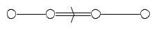
We apply the slice and projection techniques to the 52-dimensional exceptional Lie algebra \(F_4\), whose Dynkin diagram is shown in Figure 20. We number the nodes 1 through 4, from left to right, and use this numbering to label the simple roots \(r^1, \cdots, r^4\). Thus, the magnitude of \(r^1\) and \(r^2\) is greater than the magnitude of \(r^3\) and \(r^4\). We color these simple roots magenta (\(r^1\)), red (\(r^2\)), blue (\(r^3\)), and green (\(r^4\)).
 |
|
|
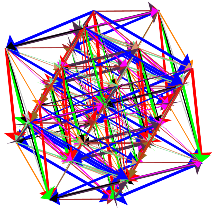
We consider the slicing of \(F_4\) defined using roots \(r^2\), \(r^3\), and \(r^4\). Laying the slices along the \(x\) axis, the large number of grey struts in the resulting diagram, Figure 21, makes it difficult to observe the underlying structure of each slice, and so they are removed from the diagram in Figure 22. This diagram clearly contains three nontrivial rank \(3\) root or weight diagrams. Comparing this diagram to the root diagrams in Figure 9, we identify the middle diagram, containing 18 non-zero vertices, as the root diagram of \(C_3=sp(2\cdot 3)\). The other two slices are identical non-minimal weight diagrams of \(C_3\). Because there are \(46\) non-zero vertices visible in Figure 22, it is clear that two single vertices are missing from this representation of the root diagram of \(F_4\), which has dimension 52.
 |
|
|
 |
|
|
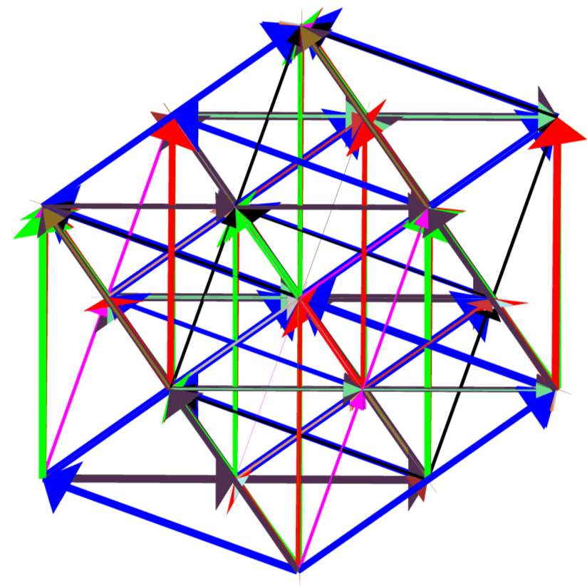
Figure 23 is the result of slicing the root diagram of \(F_4\) using the simple roots \(r^1\), \(r^2\), and \(r^3\). The center diagram again contains 18 non-zero weights, which we identify as \(B_3=so(7)\) using Figure 9. Hence, \(B_3 \subset F_4\). Furthermore, as all 48 non-zero vertices are present and there are 5 nontrivial slices in the root diagram, we compare this sliced root diagram of \(F_4\) with that of \(B_4=so(9)\), which is shown in Figure 17, and see that \(B_3 \subset B_4 \subset F_4\). An additional slicing of \(B_4\) shows \(D_4 =so(8) \subset B_4 \subset F_4\).
 |
|
|
4.2 Subalgebras of \(F_4\) using Projections
Given the 4-dimensional root diagram of \(F_4\), we can observe its \(3\)-dimensional shadow when projected along any one direction. However, as a single projection eliminates the information contained in one direction, it is not possible to understand the root diagram of \(F_4\) using a single projection. We work around this problem by creating an animation of projections, in which the direction of the projection changes slightly from one frame to the next.
The Dynkin diagram of \(F_4\) reduces to the Dynkin diagram of \(C_3=sp(2\cdot 3)\) or \(B_3=so(7)\) by eliminating either the first or fourth node. The simple roots \(r^1\) and \(r^4\) define a plane in \(\mathbb{R}^4\), and we choose a projection vector \(p_{\theta} = \cos \theta r^1 + \sin \theta r^4\) to vary discretely in steps of size \(\frac{\pi}{18}\) from \(\theta = 0\) to \(\theta = \frac{\pi}{2}\) in this plane. Each value of \(\theta\) produces a frame of the animation sequence using the projection procedures of section 3.2. The resulting animation is displayed in Figure 24.
The result of each projection of \(F_4\) is a diagram in three dimensions. We create the animation using Maple, and the software package Javaview is used to make a live, interactive applet of the animation. The Javaview applet allows the animation to be rotated in \(\mathbb{R}^3\) as it plays. In particular, when \(\theta = 0\), we can rotate the diagram to show a weight diagram of \(C_3=sp(2\cdot 3)\), which our eyes project down to the root diagram of \(B_2 = C_2\). Without rotating the diagram, the animation continuously changes the projected diagram as \(\theta\) increases. When \(\theta = \frac{\pi}{2}\), our eyes project the root diagram of \(B_3 = so(7)\) down to the root diagram of \(G_2\). However, it is also possible to rotate the animation to see the root diagram of \(G_2\) at various other values of \(\theta\). The interactive animation makes it easier to explore the structure of \(F_4\).
This interactive animation can also illustrate an obvious fact about planes in \(\mathbb{R}^4\). As \(p_{\theta}\) is confined to a plane, there is a plane \(P^{\perp}\) which is orthogonal to each of the projection directions. Thus, the projection does not affect \(P^{\perp}\), and it is possible to see this plane in \(\mathbb{R}^3\) by rotating the animation to the view shown in the sixth diagram in Figure 24. In this configuration, the roots and vertices in this diagram do not change as the animation varies from \(\theta = 0\) to \(\theta = \frac{\pi}{2}\). While this is obvious from the standpoint of Euclidean space, it is still surprising this plane can be seen in \(\mathbb{R}^3\) even as the projected diagram is continually changing.
 |
 |
 |
||
|
|
|
|
||
 |
 |
 |
||
|
|
|
|
||
|
Here is the interactive animation in a separate window. |
||||
4.3 Modifications of methods for \(E_6\)
Of particular interest is the exceptional Lie algebra \(E_6\), which preserves the the determinant of elements of the Cayley plane. As explained in Section 2.1, this allows us to write \(E_6 = sl(3,\mathbb{O})\). It therefore naturally contains the subalgebras \(sl(2,\mathbb{O})\) and \(su(2, \mathbb{O})\), which are identified as real forms of \(D_5\) and \(B_4\), respectively [13].
The projection technique can also be used to identify subalgebras of rank \(E_6\). In one version, we project the root diagram of \(E_6\) along one direction, thereby creating a diagram that possibly corresponds to a rank 5 algebra \(g\). We then apply the same pair of projections to our projected \(E_6\) diagram and to the candidate root diagram of \(g\). If these two projections preserve the number of vertices in the \(5\)-dimensional diagrams, it is possible to compare the resulting diagrams in \(\mathbb{R}^3\). If we have identified the correct subalgebra of \(E_6\), the resulting two diagrams should match for every pair of projections applied to the 5-dimensional diagrams.
Projections of rank 5 and 6 algebras can also be simulated using slicings of their root diagrams. This is done using the slice and collapse technique, which collapses all the slices onto one another in a particular direction. When using this technique, we draw the grey struts, as we are now interested in the root diagram's structure after the projection. This technique provides clearer pictures compared to the pure projection method.
4.4 Subalgebras of \(E_6\)
We list in Figure 25 the subalgebras of \(E_6\) found using the slicing and projection techniques applied to an algebra's root diagram. As mentioned in Section 2.1, we list certain real representations of the subalgebras of the \(sl(3,\mathbb{O})\) representation of \(E_6\) in the diagram. The particular real representations are listed below each algebra.
We use different notations to indicate the particular method that was used to identify subalgebras. The notation  indicates the slicing method was used to identify \(A\) as a subalgebra of \(B\). The notation
  indicates that \(A\) was identified as a subalgebra of \(B\) using the normal projection technique, while we indicate projections done by the slice and collapse method as
  . If both dotted and solid arrows are present, then \(A\) can be found as a subalgebra of \(B\) using both slicing and projection methods. If \(A\) and \(B\) have the same rank, only the slicing method allows us to identify the root diagram of \(A\) as a subdiagram of \(B\). This case is indicated in the diagram using the notation
  . Each of the subalgebra inclusions below can be verified online [14].
 |
|
|
Lists of subalgebra inclusions are found in [12], which applies subalgebras to particle physics, and in [15], which recreates the subalgebra lists of [16]. However, the list in [15] mistakenly has \(C_4\) and \(B_3\) as subalgebras of \(F_4\), instead of \(C_3\) and \(B_4\). Further, the list omits the inclusions \(G_2 \subset B_3\), \(C_4 \subset E_6\), \(F_4 \subset E_6\), and \(D_5 \subset E_6\). The correct inclusions of \(C_3 \subset F_4\) and \(B_4 \subset F_4\) are listed in Section 8 of [16], but the \(B_n\) and \(C_n\) chains are mislabeled in the final table which was used by Gilmore in [15]. Although van der Waerden uses root systems do determine subalgebra inclusions, he mistakenly claims that \(D_n \subset C_n\) as a subalgebra in Section 21, which is not true since their root diagrams are based upon inequivalent highest weights.
In [9], Dynkin classified subalgebras depending upon the root structure. If the root system of a subalgebra can be a subset of the root system of the full algebra, the subalgebra is called a regular subalgebra. Otherwise, the subalgebra is special. A complete list of regular and special subalgebras are listed in [12]. All of the regular embeddings of an algebra in a subalgebra of \(E_6\) can be found using the slicing method. In many cases, the projection technique also identifies these regular embeddings of subalgebras, but there are regular embeddings which can are not recognized as the result of projections. The special embeddings of an algebra in a subalgebra of \(E_6\) can only be found using the projection technique.
Visualizing Lie Subalgebras using Root and Weight Diagrams
5. Conclusion
We have presented here methods which illustrate how root and weight diagrams can be used to visually identify the subalgebras of a given Lie algebra. While the standard methods of determining subalgebras rely upon adding, removing, or folding along nodes in a Dynkin diagram, we show here how to construct any of a Lie algebra's root or weight diagrams from its Dynkin diagram, and how to use geometric transformations to visually identify subalgebras using those weight and root diagrams. In particular, we show how these methods can be applied to algebras whose root and weight diagrams have dimensions four or greater. In addition to pointing out the erroneous inclusion of \(C_4 \subset F_4\) in [15, 16], we provide visual proof that \(C_4 \subset E_6\) and list all the subalgebras of \(E_6\). While we are primarily concerned with the subalgebras of \(E_6\), these methods can be used to find subalgebras of any rank \(l\) algebra.
Endnotes
1There are two minimal representations of \(A_2\), only one of which is shown in Figure 2. The second minimal weight diagram of \(A_2\) is similar, but rotated \(180^\circ\) from the one shown. We omit this diagram, since it contributes no new information to the determination of subalgebras, which is our primary goal.
2For algebras of rank 6 and lower, the exceptions are that \(B_n = so(2n+1)\) and \(C_n=sp(2 \cdot n)\) have the same dimension for each rank \(n\), and that \(B_6\), \(C_6\), and \(E_6\) all have dimension 78.
3The distance between adjacent weights in the infinite lattice is less than or equal to the length of each root vector. Root vectors do not always connect adjacent weights, but often skip over them.
4 An equivalent projection \(\mathbb{R}^6 o \mathbb{R}^3: (x,y,z,u_1,u_2,u_3) o (x+s_1 u_1 + s_2 u_2 + s_3 u_3, y, z)\) with \(s_1 > \eta_2 s_2 > \eta_3 s_3\) for sufficiently large \(\eta_2\) and \(\eta_3\) will string a 6-dimensional diagram along one axis. The \(u_1\) coordinate will separate the different 5-dimensional slices, with \(s_1 u_1\) moving these different slices very apart. The \(u_2\) and \(u_3\) coordinates will locally separate the 4-dimensional and 3-dimensional slices along the \(x\) axis, but sufficiently small \(s_2\) and \(s_3\) will keep the subslices of one 5-dimensional slice from interfering with another 5-dimensional slice. This method generalizes to \(n\)-dimensional diagrams, but creates a very long string of the resulting diagrams.
5 The large number of grey lines in a diagram can hide the important roots within each slice in addition to causing computational overload.
6 While the root vectors in the octahedron and the \(C_3\) root diagram appear to intersect, they do not terminate or start from any common vertex.
References
[1] Nathan Jacobson. Lie Algebras, and Representations: An Elementary Introduction. 1st edition, 2006.
[2] J. F. Cornwell. Group Theory in Physics: An Introduction. ACADEMIC PRESS, San Diego, California, 1997.
[3] Wikipedia. Lie algebra - wikipedia, the free encyclopedia, 2006. Available at http://en.wikipedia.org/w/index.php?title=Lie_algebra&oldid=93493269 [Online; accessed 31-December-2006].
[4] Corinne A. Manogue and Jorg Schray. Finite Lorentz Transformations, Automorphisms, and Division Algebras. J. Math. Phys., 34:3746-3767, 1993.
[5] E. Corrigan and T. J. Hollowood. A String Construction of a Commutative Non-Associative Algebra related to the Exceptional Jordan Algebra. Physics Letters B, 203:47-51, March 1988.
[6] John C. Baez. The Octonions. Bull. Amer. Math. Soc., 39:145-205, 2002. Also available as http://math.ucr.edu/home/baez/octonions/.
[7] Susumu Okubo. Introduction to Octonion and Other Non-Associative Algebras in Physics. Cambridge University Press, Cambridge, 1995. See also http://www.ams.org/mathscinet-getitem?mr=96j:81052.
[8] The Atlas Project. Representations of E8, 2007. Available at http://aimath.org/E8/.
[9] E. B. Dynkin. Semi-simple subalgebras of semi-simple lie algebras. Am. Math. Soc. Trans., No. 1:1-143, 1950.
[10] J. Patera S. Kass, R. V. Moody and R. Slansky. Affine Lie Algebras, Weight Multiplicities, and Branching Rules, volume 1. University of California Press, Los Angeles, California, 1990.
[11] Zome tools. Available at http://www.zometools.com.
[12] Ulf H. Danielsson and Bo Sundborg. Exceptional Equivalences in N=2 Supersymmetric Yang-Mills Theory. Physics Letters B, 370:83, 1996. Also available as http://arXiv.org/abs/hep-th/9511180.
[13] Aaron Wangberg. The Structure of \(E_6\). Ph. D. thesis, Oregon State University, 2007.
[14] Aaron Wangberg. Subalgebras of \(E_6\) using root and weight diagrams, 2006. Available at http://oregonstate.edu/~drayt/JOMA/subalgebra_frameset.htm.
[15] Robert Gilmore. Lie Groups, Lie Algebras, and Some of Their Applications. Wiley, 1974. Reprinted by Dover Publications, Mineola, New York, 2005.
[16] B. L. van der Waerden. Die Klassifikation der einfachen Lieschen Gruppen. Mathematische Zeitschrift, 37:446-462, 1933.