- About MAA
- Membership
- MAA Publications
- Periodicals
- Blogs
- MAA Book Series
- MAA Press (an imprint of the AMS)
- MAA Notes
- MAA Reviews
- Mathematical Communication
- Information for Libraries
- Author Resources
- Advertise with MAA
- Meetings
- Competitions
- Programs
- Communities
- MAA Sections
- SIGMAA
- MAA Connect
- Students
- MAA Awards
- Awards Booklets
- Writing Awards
- Teaching Awards
- Service Awards
- Research Awards
- Lecture Awards
- Putnam Competition Individual and Team Winners
- D. E. Shaw Group AMC 8 Awards & Certificates
- Maryam Mirzakhani AMC 10 A Awards & Certificates
- Two Sigma AMC 10 B Awards & Certificates
- Jane Street AMC 12 A Awards & Certificates
- Akamai AMC 12 B Awards & Certificates
- High School Teachers
- News
You are here
Numbers and Computers

Publisher:
Springer
Publication Date:
2015
Number of Pages:
231
Format:
Hardcover
Price:
109.00
ISBN:
9783319172590
Category:
Monograph
[Reviewed by , on ]
David S. Mazel
01/27/2016
While computers are ubiquitous, are they accurate at what they do? Can we trust them to compute and work as we expect? Much of science is based on computer simulations and yet computers are, in fact, limited, prone to numerical errors (by design!), and their results require checks and re-checks. If you don’t believe this then read this book.
This book is, on one level, a discussion of how computers work with numbers. It tells how computers represent numbers such as integers, floating point numbers, big integers, decimals, and what is more, how one can write one’s own routines to operate on numbers. The book is filled with C and Python code, so the reader can implement the routines to create his own library of number manipulation subroutines, change the bit representations of numbers, and simply understand how program calls that programmers, engineers, mathematicians, etc. may take for granted, actually work. And if that’s all you want from the book, you will be quite happy. Kneusel’s writing is clear, well-organized, easy to follow, easy to implement, and a wonderful learning experience.
On a deeper level this book shows the limitations of computers. Many of us know there have always been the limits imposed by changing data types, such as floats to integers. But what about the limits of binary itself? Mr. Kneusel tells the story of how a slight numerical representation error was fatal to 28 soldiers. Here is a paraphrased version of the story:
On February 25, 1991, a scud missile hit a US Army barracks in Dharan, Saudi Arabia. The missile could have been intercepted except that the interceptor was never fired. The Patriot battery protecting the barracks failed to launch an interceptor because the computer thought the missile was out of range by about half-kilometer. The error was tracked to a small programming issue. The program kept time in steps of 0.1 seconds and used a 24-bit fixed-point float to represent that increment. However, 0.1 is not perfectly representable in binary and the error is approximately 0.000000095 seconds. If the Patriot operators would have rebooted the program frequently, this error might have been tolerable. In fact, Israeli operators of Patriot batteries noted the error accumulated to a 20% targeting error after 8-hours of operation. In this case, the Patriot system had been running for 100-hours, causing an error of 0.34 seconds and a target distance error large enough to keep the interceptor from launching. The error cost 28-soldiers their lives.
The limitations of computers can be even more subtle. Most simulations, and dynamical systems in particular, rely on feedback to generate states and evolve systems to predict future behavior. A simple dynamical system that does this is the logistic equation: \[ x_{i+1} = r x_{i}(1-x_{i}) ; i = 1, 2, \ldots, \]which you can implement easily to see the evolution of the variable \( x \). Because the logistic equation is chaotic for certain values of \( r \), initial conditions of, say, \( x_{1} = 1.5 \) or \( x_{1} = 1.50005 \) are expected to yield different trajectories. This is the idea of sensitive dependence on initial conditions, a fundamental behavior of chaotic systems.
But, what if we keep the same value for \( r \), and \( x_{1} \) and simply change the algebraic representation of the equation? Will the trajectory change? Kneusel shows it will because the computer calculation changes with a change to the equation format. To see this myself, I wrote the equations in two different ways:\[x_{i+1} = r \cdot x_{i} (1.0 - x_{i}) \] and \[x_{i+1} = r \cdot x_{i} - r \cdot x_{i} \cdot x_{i} \] Figure 1 shows the trajectory of \( x \) with \( r=10 \) and \( x_{1} = 0.1 \) where I used floats for the variables and implemented the equation with C on a Raspberry Pi computer.
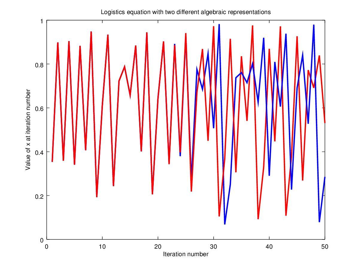
Figure 1: Logistic equation implementation in C.
The blue curve corresponds to \( x_{i+1} = r \cdot x_{i} (1.0 - x_{i}) \) and the red
curve corresponds to \( x_{i+1} = r \cdot x_{i} - r \cdot x_{i} \cdot x_{i} \).
If you write the equations in other ways (I tried six) you will see a similar divergence in the results; no two expressions give the same trajectory. This observation applies even when I used double precision for the numbers. To quote Kneusel: “Which value, if any, is most correct?” Hard to know, isn’t it? Kneusel has more to say and other examples in his book.
If this makes you wonder about the utility of computers and how to better understand numerical representations and calculations, you will do well to add this book to your winter reading list. Happy computing.
David S. Mazel is a practicing engineer in Washington, DC. He welcomes your thoughts and feedback. He can be reached at mazeld at gmail dot com.
See the publisher's page for this book.
- Log in to post comments


