- About MAA
- Membership
- MAA Publications
- Periodicals
- Blogs
- MAA Book Series
- MAA Press (an imprint of the AMS)
- MAA Notes
- MAA Reviews
- Mathematical Communication
- Information for Libraries
- Author Resources
- Advertise with MAA
- Meetings
- Competitions
- Programs
- Communities
- MAA Sections
- SIGMAA
- MAA Connect
- Students
- MAA Awards
- Awards Booklets
- Writing Awards
- Teaching Awards
- Service Awards
- Research Awards
- Lecture Awards
- Putnam Competition Individual and Team Winners
- D. E. Shaw Group AMC 8 Awards & Certificates
- Maryam Mirzakhani AMC 10 A Awards & Certificates
- Two Sigma AMC 10 B Awards & Certificates
- Jane Street AMC 12 A Awards & Certificates
- Akamai AMC 12 B Awards & Certificates
- High School Teachers
- News
You are here
Logistic Growth Model - Fitting a Logistic Model to Data, I
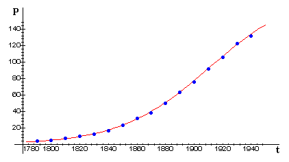
n the figure below, we repeat from Part 2 a plot of the actual U.S. census data through 1940, together with a fitted logistic curve. (Recall that the data after 1940 did not appear to be logistic.)
In this part we will determine directly from the differential equation
- how to tell whether a given set of data is reasonably logistic,
and, if so,
- what parameters r and K will give a good fit.
Our test case will be the U.S. Census data, first up to 1940, then up to 1990. In Part 6 we will study the same questions, but we will use the known form of the logistic solution from Part 4.
To determine whether a given set of data can be modeled by the logistic differential equation,
we have to estimate values of the derivative dP/dt from the data. We will do that by symmetric differences, as shown in the following figure. The slope dP/dt at a given census year t is approximated by the slope of the line joining the points 10 years earlier and 10 years later.
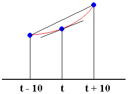
For example, the growth rate dP/dt in 1900 was approximately
Of course, for the period from 1790 through 1940, we can calculate these slope estimates only from 1800 through 1930, because we need a data point before and after each point at which we are estimating the slope.
We may rewrite the logistic equation in the form

In this form the equation says that the proportional growth rate (i.e., the ratio of dP/dt to P) is a linear function of P. Thus, we have a test of logistic behavior:
- Calculate the ratios of slopes to function values.
- Plot these ratios against the corresponding function values.
- If the resulting plot is approximately linear, then a logistic model is reasonable.
The same graphical test tells us how to estimate the parameters:
- Fit a line of the form y = mx + b to the plotted points. The slope m of the line must be -r/K and the vertical intercept b must be r.
- Take r to be b and K to be -r/m.
- Use the commands in your helper application worksheet to construct symmetric difference estimates of dP/dt for the U.S. population data, to find ratios of dP/dt to the populations P, and to plot these ratios against P. You should find that the plot is roughly linear -- but only roughly.
- Estimate the slope and vertical intercept of a line that will resonably fit the plotted points.
- Check your work by plotting r (1 - P/K) on top of the plotted points. If necessary, adjust r and/or K until you are satisfied with the fit.
- Interpret your final parameter values in terms of early growth of the U.S. population and ultimate size of the population. Are these numbers realistic? Why or why not?
- Use the next set of commands in your worksheet to extend the logistic test to U.S. population data through 1990. In what way does the plot tell you that a logistic model for this data would not be reasonable?
Leonard Lipkin and David Smith, "Logistic Growth Model - Fitting a Logistic Model to Data, I," Convergence (December 2004)


